The Design of an Experiment
The way that a sample is selected is called the
sampling plan or
experimental design. The sampling plan determines how much information is gathered in the sample. Some research involves an
observational study, in which the researcher does not actually produce the data but only observes the characteristics of data that already exist. Most sample surveys, in which information is gathered with a questionnaire, fall into this category. The researcher forms a plan for collecting the data—called the sampling plan—and then uses the appropriate statistical procedures to draw conclusions about the population or populations from which the sample comes.
Other research involves
experimentation. The researcher may deliberately impose one or more experimental conditions on the experimental units in order to determine their effect on the response. Here are some new terms we will use to discuss the design of a statistical experiment.
Definitions
An experimental unit is the object on which a measurement (or measurements) is taken.
A factor is an independent variable whose values are controlled and varied by the experimenter.
A level is the intensity setting of a factor
A treatment is a specific combination of factor levels
The response is the variable being measured by the experimenter
Example
A group of golfers who all have the same handicap (they all typically score the same) is randomly divided into an experimental and control group. The control group is asked to golf 18 holes and record their scores after having eaten a full breakfast. The experimental group is asked to golf 18 holes at the same time as the control group, and record their scores, without having eaten any breakfast. What are the factors, levels and treatments in this experiment?
Solution
The
experimental units are the people on which the
response (golf score) is measured. The
factor of interest could be described as a 'meal' and has two
levels: 'breakfast' and 'no breakfast.' Since this is the only factor controlled by the experimenter, the two levels — 'breakfast' and 'no breakfast' —also represent the
treatments of interest in the experiment.
Example
Suppose the experimenter in the previous example began by randomly selecting 30 golfers aged 20 to 29 and 30 golfers aged 30 to 39 for the experiment. These two groups were then randomly divided into 15 each for the experimental and control groups. What are the factors, levels and treatments?
Solution
Now there are two
factors of interest to the experimenter, and each factor has two levels:
- 'age' at two levels: ages 20 to 29 and ages 30 to 39
- 'meal' at two levels: breakfast and no breakfast
In this more complex experiment, there are four
treatments, one for each specific combination of factor levels: golfers ages 20 to 29 with no breakfast, golfers ages 20 to 29 with breakfast, golfers ages 30 to 39 with no breakfast and golfers ages 30 to 39 with breakfast.
In this section, we will concentrate on an experiment that involves one factor set at $k$ levels, and we will use a technique called the
analysis of variance to judge the effects of that factor on the experimental response.
What is an Analysis of Variance?
The responses that are generated in an experimental situation always exhibit a certain amount of
variability. In an
analysis of variance, you divide the total variation in the response measurements into portions that may be attributed to various factors of interest to the experimenter. If the experiment has been properly designed, these portions can then be used to answer questions about the effects of the various factors on the response of interest.
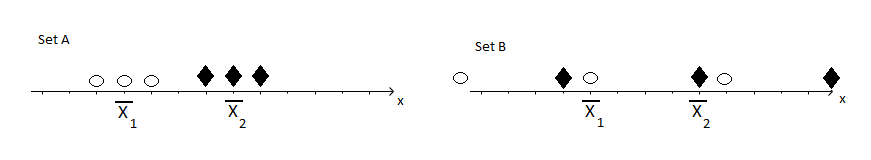
You can better understand the logic underlying an analysis of variance by looking at a simple experiment. Consider two sets of samples randomly selected from populations 1 (white ovals) and 2 (black triangles), each with the same number of pairs of means, $\bar{x_1}$ and $\bar{x_2}$. The two sets are shown in the figure below.
Is it easier to detect the difference in the two means when you look at set A or set B? You will probably agree that set A shows the difference much more clearly. In set A, the variability of the measurements
within the respective groups (black triangles and white ovals) is much smaller than the variability
between the two groups. In set B, there is more variability
within the groups (black triangles and white ovals) causing the two groups to 'mix' together and making it more difficult to see the
identical difference between the means.
The comparison you have just done intuitively is formalized by the analysis of variance. Moreover, the analysis of variance can be used not only to compare two means but also to make comparisons of more than two population means and to determine the effects of various factors in more complex experimental designs. The analysis of variance relies on statistics with sampling distributions that are modeled by the F distribution of Secion 10.3 in your textbook.
The Assumptions for an Analysis of Variance
The assumptions upon which the test and estimation procedures for an analysis of variance are based are similar to those required for the Student's t and F statistics from chapters 7, 8 and 10. Regardless of the experimental design used to generate the data, you can assume that the observations within each treatment group are normally distributed with a common variance, $\sigma^2$. The analysis of variance procedures are fairly robust when the sample sizes are equal and when the data are fairly bell shaped. Violating the assumptions of a common variance is more serious, especially when the sample sizes are not nearly equal.
Definitions
Assumptions for Analysis of Variance Test and Estimation Procedures
- The observations within each population are normally distributed with a common variance, $\sigma^2$
- Assumptions regarding the sampling procedure are specified for each experimental design.
This section describes the analysis of variance for one simple experimental design. This design is based on independent random sampling from several populations and is an extension of the unpaired $t$ test from chapter 8 (section 2).
The Completely Randomized Design: A One-Way Classification
One of the simplest experimental designs is the
completely randomized design, in which random samples are selected independently from $k$ populations. This design involves only one
factor, the population from which the measurements comes — hence the designation as a
one -way classification. There are $k$ different
levels corresponding to $k$ populations, which are also treatments for this one-way classification. Are the $k$ population means all the same, or is at least one mean different from the others?
Why do you need a new procedure, the
analysis of variance, to compare the population means when you already have the Student's t test available? In comparing $k=3$ means, you could test each of three pairs of hypotheses:
$$
H_0: \mu_1=\mu_2 \qquad H_0: \mu_1=\mu_3 \qquad H_0: \mu_2=\mu_3 \qquad
$$
to find out where the differences lie. However, you must remember that each test you perform is subject to the possibility of error. To compare $k=4$ means, you would need six tests, and you would need ten tests to compare $k=5$ means. The more tests you perform on a set of measurements, the more likely it is that at least one of your conclusions will be incorrect. The analysis of variance procedure provides one overall test to judge the equality of $k$ population means. Once you have determined whether there is actually a difference in the means, you can use another procedure to find out where the differences lie.
How can you select these $k$ random samples? Sometimes the populations actually exist in fact, and you can use a computerized random number generator or a random number table to randomly select the samples. For example, in a study to compare the average sizes of health insurance claims in four different states, you could use a computer database provided by the health insurance companies to select random samples from the four states.
Example
A researcher is interested in the effects of five types of insecticide for use in controlling the boll weevil in cotton fields. Explain how to implement a completely randomized design to investigate the effects of the five insecticides on crop yield.
Solution
The only way to generate the equivalent of five random samples from the hypothetical populations corresponding to the five insecticides is to use a method called randomized assignment. A fixed number of cotton plants are chosen for treatment, and each is assigned a random number. Suppose that each sample is to have an equal number of measurements. Using a randomization device, you can assign the first $n$ plants chosen to receive insecticide 1, the second $n$ plants to receive insecticide 2, and so on, until all five treatments have been assigned.
Whether by random selection or random assignment, both of these examples result in completely randomized design, or one-way classification, for which the analysis of variance is used.
The Analysis of Variance for a Completely Randomized Design
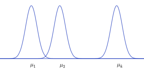
Suppose you want to compare $k$ population means, $\mu_1, \mu_2, ..., \mu_k,$ based on independent random samples of size $n_1, n_2, ..., n_k$ from normal populations with a common variance, $\sigma^2$. That is, each of the normal populations has the same shape but their locations migh be different, as shown in the figure below.
Partitioning the Total Variation in an Experiment
Let $x$ be the variable representing the list of all measurements taken from all $k$ samples. Also let $\bar{\bar{x}}$ represent the mean of all measurements from all $k$ samples. That is, $\bar{\bar{x}} = \dfrac{\sum x }{ n}.$ The analysis of variance procedure begins by examining the total variation in the experiment, which is measured by a quantity called the
total sum of squares:
$$\text{Total SS} = \sum(x-\bar{\bar{x}})^2 = \sum x^2 - \frac{(\sum x)^2}{n}$$
$\sum(x-\bar{\bar{x}})^2$ is the familiar numerator in the formula for the sample variance for the entire set of $n$ measurements ($n=n_1+n_2+\dots+n_k$). The second part of the calculational formula is sometimes called the
correction for the mean (abbrievated as CM in the formulas below). If we let $G$ represent the grand total of all $n$ observations, then
$$CM = \frac{(\sum x)^2}{n} = \frac{G^2}{n}$$
This Total SS is partitioned (split) into two components. The first component, called the
sum of squares for treatments ($SS_B$), measures the variation
between the $k$ sample means
$$SS_B = \sum n_i(\bar{x_i}-\bar{\bar{x}})^2 = \sum\frac{T_i^2}{n_i}-CM $$
where $T_i$ is the total of the observations for treatment $i$, and $\bar{x}_i$ is the mean of sample $i$. The second component of the Total SS, called the
sum of squares for error ($SS_W$), is used to measure the pooled variation
within the $k$ samples:
$$ SS_W = (n_1-1)s_1^2 + (n_2-1)s_2^2 + \dots +(n_k-1)s_k^2 = \sum (n_i-1)s_i^2 $$
This formula is a direct extenstion of the numerator in the formula for the pooled estimate of $\sigma^2$ from chapter 8, section 2. We can show algebraically that, in the analysis of variance,
$$\text{Total SS} = SS_B+SS_W $$
Therefore, you need to calculate only two of the three sums of squares—Total SS, $SS_B$ and $SS_W$—and the third can be found by subtraction.
Each of the sources of variation, when divided by its appropriate degrees of freedom, provides an estimate of variation in the experiment. Since Total SS involves n squared observations, its degrees of freedom are $df=(n-1)$. Similarly, the sum of squares for treatments involves $k$ squared observations, and so it's degrees of freedom are $df=(k-1)$. Finally, the sum of squares for error, a direct extension of the pooled estimate in Chapter 8 has
$$df= (n_1-1)+(n_2-1)+\dots+(n_k-1)=n-k$$
Notice that the degrees of freedom for treatments and error are additive—that is
$$df(total)= df(treatments)+df(error)$$
These two sources of variation and their respective degrees of freedom are combined to form the mean squares as
$\text{MS}=\frac{\text{SS}}{df}$. The total variation in the experiment (of the list of all n measurements in the experiment)
$$ Total \ Sample \ Variation= \frac{\sum(x-\bar{\bar{x}})^2}{n-1} = \frac{SS_B+SS_W}{(k-1)+(n-k)} $$
is then displayed (in parts) in an
analysis of variance (or ANOVA) table.
ANOVA Table for $k$ Independent Random Samples: Completely Randomized Design
$$
\begin{array}{c|c|c|c|c}
\color{blue}{Variation \ Source} & \color{blue}{ df } & \color{blue}{ Sum \ of \ Squares (SS) } & \color{blue}{Mean \ of \ Squares (MS)} &\color{blue}{F} \\\hline
Treatments & k-1 & SS_B& MS_B& MS_B/MS_W\\
Error & n-k & SS_W & MS_W&\\ \hline
Total & n-1 & Total \ SS & &
\end{array}
$$
Where
$$\begin{align*}
Total \ SS & = \sum x^2 -CM \\
&\\
& = (\text{sum of squares of all x values}) - CM
\end{align*}$$
with
$$
\begin{array}{cccc}
CM = \dfrac{(\sum x)^2}{n} = \dfrac{G^2}{n} &&&\\
& & &\\
SS_B = \sum\dfrac{T_i^2}{n_i}-CM & & & MS_B=\dfrac{SS_B}{k-1} \\
& & &\\
SS_W = Total \ SS - SS_B &&& MS_W=\dfrac{SS_W}{n-k} \\
\end{array}
$$
and
$$\begin{align*}
G & = \text{Grand total of all $n$ observations}\\
T_i &= \text{Total of all observations in sample $i$}\\
n_i &= \text{Number of observations in sample $i$}\\
n &= n_1+n_2+\dots+n_k\\
\end{align*}$$
Example
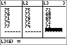
In an experiment to determine the effect of nutrition on the scores of golfers, a group of 15 golfers who all scored 72 on average were randomly assigned to each of three meal plans: no breakfast, light breakfast and full breakfast. Their scores were recorded during a morning round of golf and are shown in the table below. Construct the analysis of variance table for this experiment. Note: in golf the lowest score is the best score.
$$
\begin{array}{ccc}
No \ Breakfast & Light \ Breakfast & Full \ Breakfast\\\hline
75 & 75 & 72 \\
76 & 73 & 68 \\
71 & 76 & 69 \\
74 & 72 & 72 \\
77 & 74 & 71 \\ \hline
T_1=373& T_2=370 & T_3=352 \\
\end{array}
$$
Solution
There are $k=3$ treatments with each sample size equaling 5 (that is, $n_1=n_2=n_3=5$), the total number of measurements is $n=n_1+n_2+n_3=15$ and the sum total of all the measurements is $\sum x = T_1+T_2+T_3=1095$. Then
$$CM = \frac{1095^2}{15}=79,935$$
\begin{align*}
Total \ SS & = (75^2+76^2+71^2+\dots75^2)-CM\\
& =80,031-79,935\\
& =96\\
\end{align*}
with $(n-1)=15-1=14$ degrees of freedom. Next,
\begin{align*}
SS_B & = \sum\frac{T_i}{n_i}-CM\\
& = \biggr(\frac{373^2}{5}+\frac{370^2}{5}+\frac{352^2}{5} \biggr)-79,935\\
& =51.6\\
\end{align*}
with $(k-1)=3-1=2$ degrees of freedom. Using subtraction,
\begin{align*}
SS_W & = Total \ SS - SS_B\\
& = 96-51.6\\
&=44.4
\end{align*}
with $(n-k)=15-3=12$ degrees of freedom. Then,
\begin{align*}
MS_B & =\frac{SS_B}{k-1}\\
& =\frac{51.6}{2}\\
& = 25.8\\
\end{align*}
and
\begin{align*}
MS_W & =\frac{SS_W}{n-k}\\
& =\frac{44.4}{12}\\
& = 3.7\\
\end{align*}
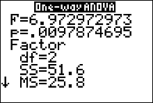
Finally, $F=\frac{MS_B}{MS_W}=\frac{25.8}{3.7}=6.729729729...$
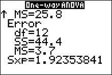
The ANOVA Table
\begin{array}{c|c|c|c|c}
\color{blue}{Variation \ Source} & \color{blue}{ df } & \color{blue}{ Sum \ of \ Squares (SS) } & \color{blue}{Mean \ of \ Squares (MS)} &\color{blue}{F} \\\hline
Treatments & k-1=2 & SS_B=51.6& MS_B=25.8& MS_B/MS_W=6.973\\
Error & n-k=12 & SS_W=44.4 & MS_W=3.7&\\ \hline
Total & n-1 & Total \ SS =96 & &
\end{array}
Table Check
As a check, we can verify that $s_x$ (the sample standard deviation from all 15 measurements in the experiment) is equal to the same number we get from taking the square root of $\frac{SS_B+SS_W}{(k-1)+(n-k)}$. That is, we need to verify that the two formulas
$$ s_x = \sqrt{\frac{SS_B+SS_W}{(k-1)+(n-k)} }$$ and
$$ s_x = \sqrt{\frac{\sum(x-\bar{\bar{x}})^2}{n-1}} $$
give the same number. If they don't equal, then we made a mistake somewhere and need to check our math and find our mistake. Another way to do the problem is to employ technology, such as a graphing calculator or statistical software.
Notice that
\begin{align*}
s_x & = \sqrt{\frac{SS_B+SS_W}{(k-1)+(n-k)} }\\
& = \sqrt{\frac{51.6+44.4}{2+12} }\\
& = \sqrt{\frac{96}{14}}\\
& = 2.618614683\\
\end{align*}
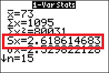
We can get the calculator to evaluate the formula
$$ s_x = \sqrt{\frac{\sum(x-\bar{\bar{x}})^2}{n-1}} $$
for us. All we need to do is enter all 15 measurements from the experiment into our calculator's list one (L1), then run the $1-var-stats$ algorithm on L1.
Below is the calculator display we should get.
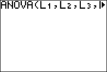
How to get the Table with the Calculator
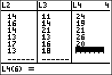
- Enter the data into L1, L2, L3, etc.
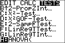
- Press STAT and move the cursor to TESTS.
- Arrow Up/Down until the cursor highlights ANOVA. Press ENTER.
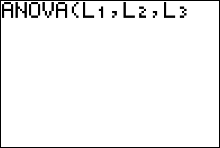
- Type each list followed by a comma. End with ) and press ENTER.
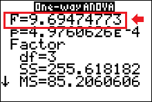
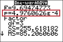
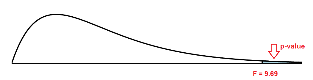
 The test statistic is $F=9.69$.