Statistical Inference

 

Statistical inference is concerned with making decisions or predictions about parameters — the numerical measures that characterize a population. Three parameters you encountered in earlier chapters are the population mean $\mu$, the population standard deviation $\sigma$, and the binomial proportion, $p$.

Methods of Statistical Inference

• Estimation:   Estimating or predicting the value of the parameter
• Hypothesis testing:   Making a decistion about the value of a parameter based on some preconceived idea about what its value might be

Types of Estimators

To estimate the value of a population parameter, you can use the information from the sample in the form of an estimator. Estimators are calculated using information from the sample observations, and so estimators are themselves statistics.

Estimators are used in two different ways:

• Point estimation:   Based on sample data, a single number is calculated to estimate the population parameter. The rule or formula that describes this calculation is called the point estimator, and the resulting number is called a point estimate.
• Interval estimation: Based on sample data, two numbers are calculated to form an interval within which the parameter is expected to lie. The rule or formula that describes this calculation is called the interval estimator, and the resulting pair of numbers is called an interval estimate or confidence interval.

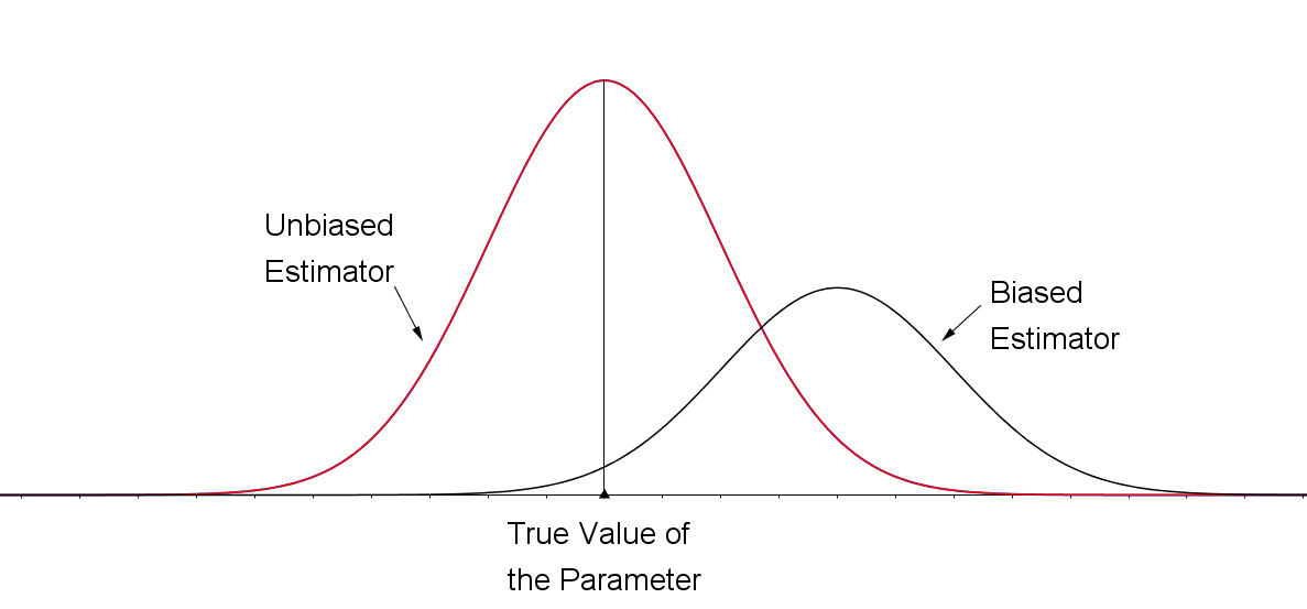
For a statistical point estimator, the sampling distribution of the estimator provides information about the best estimator. Two characteristics are valuable in a point estimator. First, the sampling the distribution of the point estimator should be centered over the true value of the parameter to be estimated. That is, the estimator should not consistently underestimate or overestimate the parameter of interest. Such an estimator is said to be unbiased.

The sampling distributions for an unbiased estimator and a biased estimator are shown in the figure. The sampling distribution for the biased estimator is shifted to the right of the true value of the parameter. This biased estimator is more likely than an unbiased one to overestimate the value of the parameter.

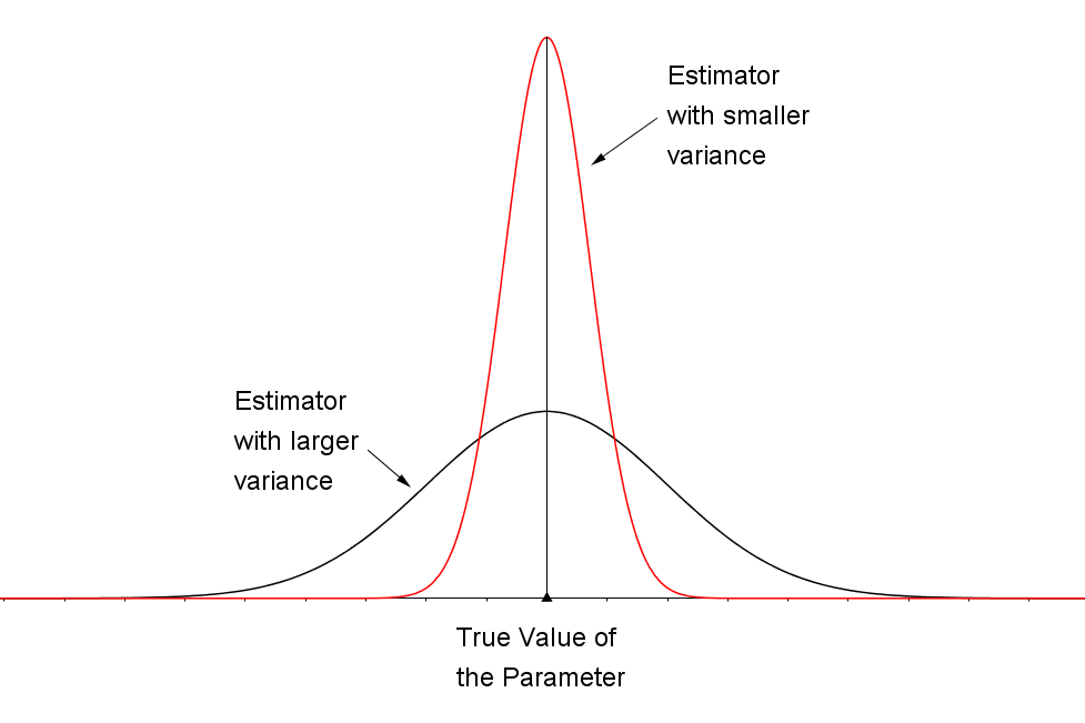
The second desirable characteristic of an estimator is that the spread (as measured by the variance) of the sampling distribution should be as small as possible. This ensures that, with a high probability, an individual estimate will fall close to the true value of the parameter. The sampling distributions for two unbiased estimators, one with a small variance and the other with a larger variance, are shown in the figure below. Naturally, you would prefer the estimator with the smaller variance because the estimates tend to lie closer to the true value of the parameter than in the distribution with the larger variance.

The Margin of Error

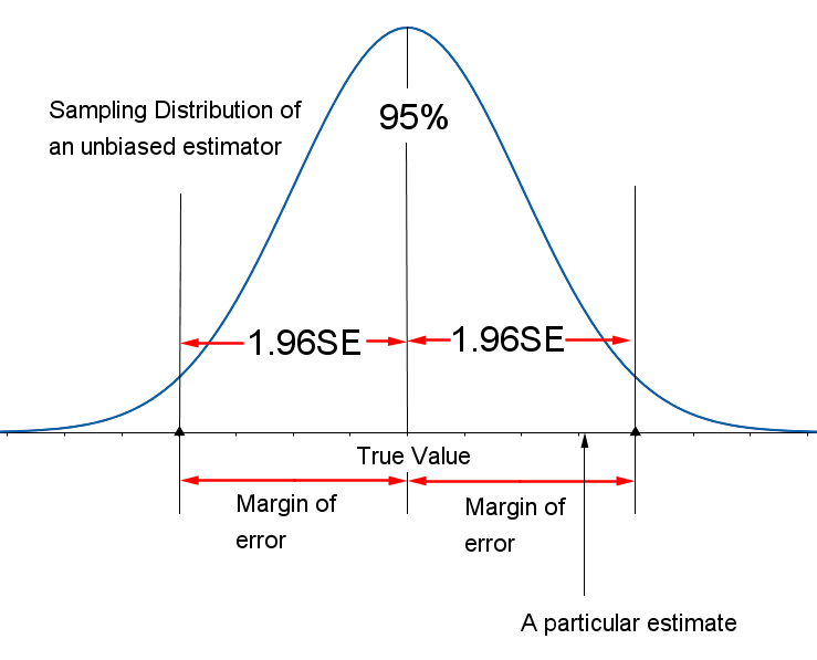
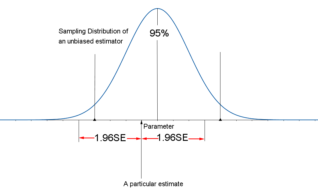
In real-life sampling situations, you may know that the sampling distribution of an estimator centers about the parameter that you are attempting to estimate, but all you have is the estimate computed from the n measurements contained in the sample. How far from the true value of the parameter will your estimate lie? How close is the marksman's bullet to the bull's-eye? The distance between the estimate and the true value of the parameter is called the error of estimation.

 

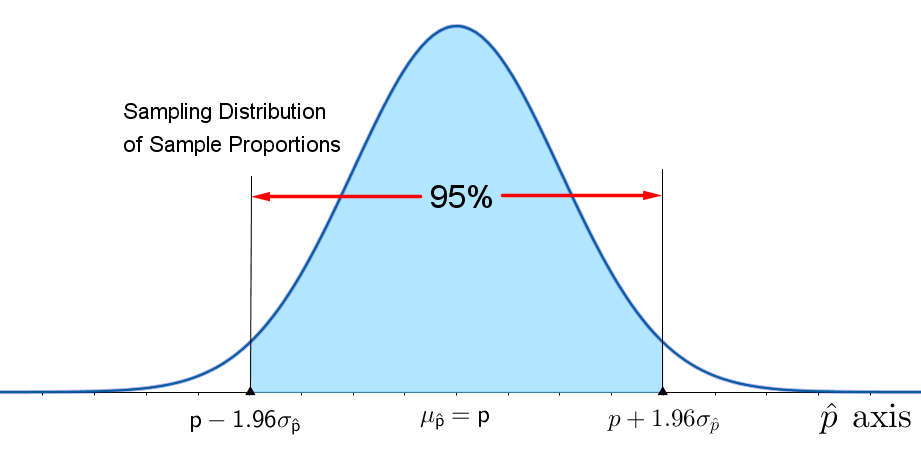
For the work we do, you may assume that the sample sizes are always large and, therefore, that the unbiased estimators you will study have sampling distributions that can be approximated by a normal distribution (because of the Central Limit Theorem). Remember that, for any point estimator with a normal distribution, the Empirical Rule states that approximately 95% of all the point estimates will lie within two (or more exactly, 1.96) standard deviations of the mean of that distribution. For unbiased estimators, this implies that the difference between the point estimator and the true value of the parameter will be less than 1.96 standard deviations or 1.96 standard errors (SE), and this quantity, called the margin of error (E), provides a practical upper bound for the error of estimation (see the figure below). It is possible that the error of estimation will exceed this margin of error (E), but that is very unlikely.

The sampling distributions for the two unbiased point estimators, \( \bar{x} \) and \( \hat{p} \) were discussed earlier. It can be shown that both of these point estimators have the minimum variability of all unbiased estimators and are thus the best estimators you can find in each situation.




When you sample a normal distribution, the statistic $\dfrac{\bar{x}-\mu}{\frac{s}{\sqrt{n}}}$ has a t distribution, which will be discussed later. When the sample is large, this statistic is approximately normally distributed whether the sampled population is normal or nonnormal.

You should notice that in calculating the standard errors for these two point estimates, you needed to estimate $\sigma$ with $s$, $p$ with $\hat{p}$ and $q$ with $\hat{q}$. These approximate standard errors will differ only slightly from the true value of SE when the sample size $n$ is large, and they will have little effect on the margin of error. In fact the table below shows that, for most values of $p$ — especially when $p$ is between 0.3 and 0.7 — there is very little change in $\sqrt{pq}$, the numerator of SE, as $p$ changes.

$p$	$pq$	$\sqrt{pq}$
0.1	0.09	0.30
0.2	0.16	0.40
0.3	0.21	0.46
0.4	0.24	0.49
0.5	0.25	0.50
0.6	0.24	0.49
0.7	0.21	0.46
0.8	0.16	0.40
0.9	0.09	0.30

Example:   A marketing analyst wants to estimate the average amount spent by a dating site customer per year. A random sample of $n=50$ dating site customers were polled about the amount they spend each year on dating websites. The results of the poll produced a mean amount of $\$240$ with a standard deviation of $\$20$. Use this information to estimate the population mean amount spent by a dating website customer per year.

Solution:   The random variable is the amount spent by a dating site customer per year. The point estimate of $\mu$ is $\bar{x}=\$240$. The margin of error is \[ 1.96\cdot SE = 1.96\cdot\sigma_{\bar{x}}=1.96\cdot\frac{\sigma}{\sqrt{n}}=1.96\cdot\frac{\sigma}{\sqrt{50}} \] Since the sample size is large (greater than 30) the analyst can approximate the value of $\sigma$ with $s$. Therefore, the margin of error is approximately \[ 1.96\cdot\frac{s}{\sqrt{n}}=1.96\cdot\frac{20}{\sqrt{50}}\doteq\$5.54 \] The analyst can feel fairly confident that the sample estimate of $\$240$ is within $\$5.54$ of the population mean.

---

Example:   In early April 2014, a major security flaw affecting perhaps 500,000 or more websites was announced and fixed. But the patch to the "secure socket" program that is supposed to encrypt and protect user information on secure websites was only made after more than two years of vulnerability on some of the most heavily trafficked sites, including Facebook, Google, YouTube, Yahoo and Wikipedia. Analysts warned that untold numbers of internet users might have had key personal information compromised either in their use of those websites, or their use of email, instant messaging, and even supposedly secure virtual personal networks.

The software bug was named "Heartbleed" and it was accidentally introduced to the OpenSSL encryption program on New Year’s Eve 2011. Some security commentators called Heartbleed "catastrophic" and said it was one of the worst vulnerabilities ever discovered on the web. Shortly after the bug, a researcher was interested in determining the percentage of people who changed their passwords or cancelled accounts. A random sample of 1501 internet users were polled and 39% of those polled indicated they had changed their passwords or cancelled accounts since the announcement of "Heartbleed." Use this information to estimate the true population proportion of adults who changed their passwords or cancelled accounts since the announcement of "Heartbleed," and find the margin of error for the estimate.

Solution:   The best estimator of the population proportion $p$ is the sample proportion $\hat{p}$, which for this sample is $\hat{p}=0.39$. In order to find the margin of error you can approximate the value of $p$ with its estimate $\hat{p}=0.39=39\%$. Then: \[ 1.96\cdot SE = 1.96\cdot\sqrt{\frac{pq}{n}}\approx1.96\cdot\sqrt{\frac{\hat{p}\hat{q}}{n}}=1.96\cdot\sqrt{\frac{0.39\cdot0.61}{1501}}\doteq0.025=2.5\% \] With this margin of error you can be fairly confident that the estimate of 39% is within $\pm2.5\%$ of the true value of $p$. You can conclude the true value of $p$ could be as low as 36.5% or as high as 41.5%. The margin of error is quite small and reflects the fact that large sample sizes are required to achieve a small margin of error.

---

As you saw in the table above the margin of error using the estimator $\hat{p}$ is a maximum when $p=0.5$. Some pollsters routinely use the maximum margin of error when estimating $p$, in which case they calculate \[ 1.96\cdot SE = 1.96\cdot\sqrt{\frac{0.5\cdot0.5}{n}} \] or sometimes \[ 2SE = 2\cdot\sqrt{\frac{0.5\cdot0.5}{n}} \] Gallup, Harris and Roper polls generally use sample sizes of approximately 1000, so their margin of error is \[ 1.96\cdot SE = 1.96\cdot\sqrt{\frac{0.5\cdot0.5}{1000}}=1.96(0.016)=0.031 \] or approximately 3%. In this case the estimate is said to be within $\pm3$ percentage points of the true population proportion.

---

Confidence Intervals

Each time you draw a sample and construct a confidence interval for a parameter, you hope to include the parameter in your interval, but, sometimes you miss. Your "success rate" — the percentage of intervals that include the parameter in repeated sampling —is the confidence level.

Level of Confidence

When the sampling distribution of a point estimator is approximately normal, an interval estimator or confidence interval can be constructed using the following reasoning. For simplicity, assume that the level of confidence is 0.95 and refer to the figure below.

• For the standard normal random variable z, 95% of all values lie between 1.96 and 1.96.
• For an unbiased point estimator with a normal sampling distribution, 95% of all point estimates lie within 1.96 standard errors of the parameter of interest.
• Consider constructing the interval as (point estimate $\pm$ 1.96$\cdot$SE). As long as the point estimate is within 1.96$\cdot$SE of the parameter of interest, the interval centered at this estimate will contain the parameter of interest. This will happen 95% of the time.

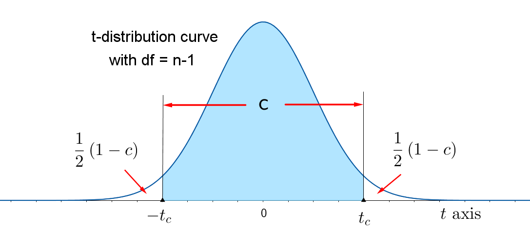
You may want to change the level of confidence from $c = 0.95$ to an­ other confidence level, $c$. When you change $c$ to something other than 95%, a value different from $z = 1.96$ will need to be used to find the Margin of Error. You will need to change the value of $z = 1.96$ — which locates an area 0.95 in the center of the standard normal curve — to a value of z that locates the area $c$ in the center of the curve, as shown in the figure below. Since the total area under the curve is 1, the remaining area in the two tails is $1-c$, and each tail contains area $\dfrac{1}{2}(1-c)$. Then $c$ is the percent of the area under the normal curve between $-z_{c}$ and $z_{c}$.

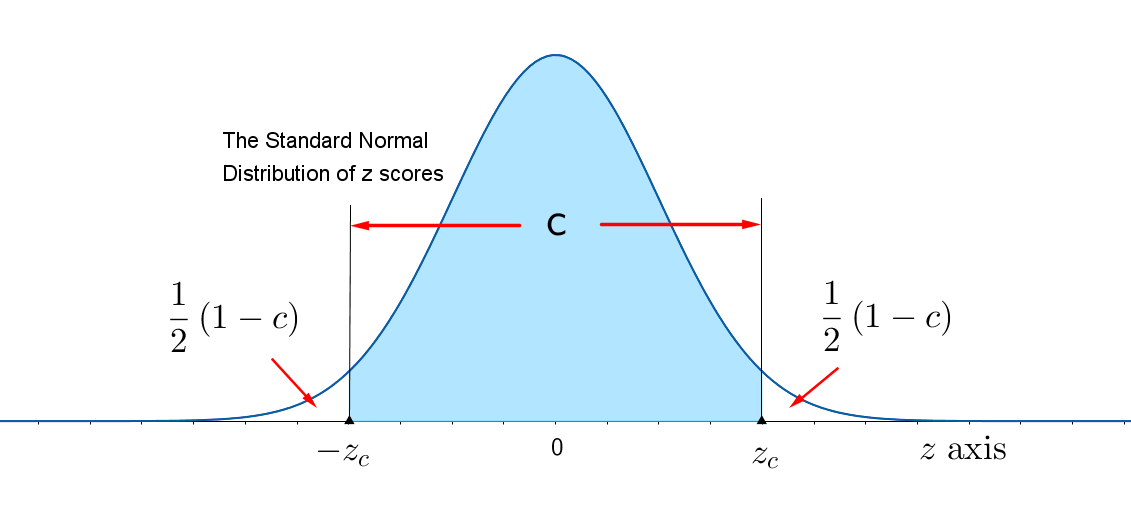
The value of $z$ that has "tail area" $\dfrac{1}{2}(1-c)$ to its right is called $z_{c}$ and the area between $-z_{c}$ and $z_{c}$ is the level of confidence $c$.   Values of $z_{c}$ that are typically used by experimenters will become familiar to you as you begin to construct confidence intervals for different practical situations. Some of these values are given in the table below.

Common Critical Values

Confidence Level $c$	$1-c$	$z_{c}$
0.90	0.10	1.645
0.95	0.05	1.96
0.98	0.02	2.33
0.99	0.01	2.58

---

Confidence Intervals for the Population Mean, $\mu$ (Large Samples)

Practical problems very often lead to the estimation of $\mu$, the mean of quantitative measurements. Here are some examples:

• The average revenue expected for San Diego County during MLB All-Star Week (2016)
• The average response time for an emergency 911 call in a particular city
• The average demand for a service

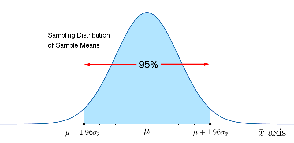
When the sample size $n$ is large, the sample mean $\bar{x}$ is the best point estimate for the population mean, $\mu$. Since the sampling distribution of sample means is approximately normal, it can be used to construct a confidence interval according to the general approach given earlier.

Here is where the formula comes from: the Central Limit Theorem tells us the sampling distribution of sample means is bell-shaped. Then the Empirical Rule tells us that 95% of sample means will be within 1.96 standard errors away from $\mu$, or that \[ P\biggr( \mu - 1.96\frac{\sigma}{\sqrt{n}} < \bar{x} < \mu + 1.96\frac{\sigma}{\sqrt{n}} \biggr) = 0.95 \] If you change the value of $z=1.96$ to $z_{c}$, then \[ P\biggr( \mu - z_{c}\frac{\sigma}{\sqrt{n}} < \bar{x} < \mu+ z_{c}\frac{\sigma}{\sqrt{n}} \biggr) = c \] This last probability statement says that a randomly selected $\bar{x}$ will be within $z_{c}$ standard errors away from the population mean with a frequency of $c$%. You can rewrite this inequality as \[ -z_{c}\frac{\sigma}{\sqrt{n}} < \bar{x}-\mu < z_{c}\frac{\sigma}{\sqrt{n}} \] if you subtract $\mu$ from all three parts of the inequality. Afterwards, we subtract $\bar{x}$ from all three parts of the inequality to get \[ -\bar{x}- z_{c}\frac{\sigma}{\sqrt{n}} < -\mu < -\bar{x}+ z_{c}\frac{\sigma}{\sqrt{n}} \] Then we multiply the inequality by $(-1)$ \[ \bar{x} + z_{c}\frac{\sigma}{\sqrt{n}} > \mu > \bar{x}- z_{c}\frac{\sigma}{\sqrt{n}} \] and change the direction of the inequality symbols. Now we can reverse the inequality direction using the symmetry property of inequalities ( i.e., since $a>b>c$ is equivalent to $c$ < $b$ < $a$) and write \[ \bar{x} - z_{c}\frac{\sigma}{\sqrt{n}} < \mu < \bar{x}+ z_{c}\frac{\sigma}{\sqrt{n}} \] so that \[ P\biggr( \bar{x} - z_{c}\frac{\sigma}{\sqrt{n}} < \mu < \bar{x}+ z_{c}\frac{\sigma}{\sqrt{n}} \biggr)=c \] Both $\bar{x} - z_{c}\frac{\sigma}{\sqrt{n}}$ and $\bar{x}+ z_{c}\frac{\sigma}{\sqrt{n}}$, the lower and upper confidence limits, are actually random quantities that depend on the sample mean $\bar{x}$. Therefore, in repeated sampling, the random interval, $\bar{x}\pm z_{c}\frac{\sigma}{\sqrt{n}}$, will contain the population mean $\mu$ with probability $c$.

---

Example:  Suppose that for a random sample of 50 computers at a certain electronics store, the mean repair cost was $\$167$. Assume the population standard deviation was $\$26$. Construct a 95% confidence interval estimate for the population mean repair cost.

Solution:   The random variable, $x$, represents the cost, in dollars, of a computer repair. The point estimate of $\mu$ is $\bar{x}=\$267$. The margin of error is \[ E=1.96\cdot SE = 1.96\sigma_{\bar{x}}= 1.96\frac{\sigma}{\sqrt{n}}=1.96\frac{26}{\sqrt{50}}\doteq\$7.21 \] The approximate 95% confidence interval is \[ \eqalign{ \bar{x} & \pm \ E\cr \bar{x} & \pm \ z_{c}\biggr( \frac{\sigma}{\sqrt{n}} \biggr)\cr \$267 & \pm \ 1.96\biggr( \frac{\$26}{\sqrt{50}} \biggr)\cr \$267 & \pm \ \$7.21 } \] The 95% confidence interval for $\mu$ is from $\$259.79$ to $\$274.21$.

---

Try This!!

Suppose that for a random sample of 120 TVs at a certain electronics store, the mean repair cost was $\$220$. Assume the population standard deviation was $\$16$. Construct a 95% confidence interval estimate for the population mean repair cost.

---

Interpreting Confidence Intervals

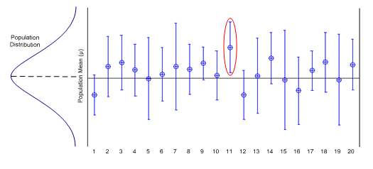
What does mean it mean to say you are "95% confident" that the true value of the population mean $\mu$ is within a given interval? If you were to construct 20 such intervals, each using different sample information, your intervals might look like those shown in the figure below. Of the 20 intervals, you might expect that 95% of them, 19 out of 20, will perform as planned and contain $\mu$ within their upper and lower bounds. Remember that you cannot be absolutely sure that any one particular interal contains the mean $\mu$. You will never know whether your particular interval is the one out of the 19 that "worked," or whether it is the one interval that "missed." Your confidence in the estimated interval follows from the fact that when repeated intervals are calculated, 95% of these intervals will contain $\mu$.

A good confidence interval has two desirable characteristics:

• It is as narrow as possible. The narrower the interval, the more exactly you have located the estimated parameter.
• It has a large level of confidence, near 100%. The larger the confidence level, the more likely it is that the interval will contain the estimated parameter.

---

Example:   A researcher wants to estimate the average amount of time, in hours per day, that a U.S. teenager spends consuming media — watching TV, listening to music, surfing the Web, social networking, and playing video games. A random sample of $n=1000$ U.S. teenagers were polled about the amount of time they spend daily consuming media. The results of the poll produced a mean amount of $7.6$ hours with a standard deviation of 2.2 hours. Use this information to estimate the population mean. Use a 90% level of confidence. (Source: The Washington Post)

Solution:   The random variable, $x$ represents the time, in hours per day, that a U.S. teenager spends consuming media. The point estimate of $\mu$ is $\bar{x}=7.6$. The critical value of $z_{c}$ can be found on the table of common values. (Alternatively, we could use the calculator, $z_{c}=invnorm\Bigg(\dfrac{1}{2}(1+c)\Bigg)=1.645$  with $c=0.90$.) The margin of error is \[ E=1.645\cdot SE = 1.645\cdot\sigma_{\bar{x}}= 1.645\cdot\frac{\sigma}{\sqrt{n}} \] Since the sample size is large (greater than 30) the researcher can approximate the value of $\sigma$ with $s$. Therefore, the margin of error is approximately \[ E=1.645\cdot SE \doteq 1.645\cdot\frac{s}{\sqrt{n}}=1.645\cdot\frac{2.2}{\sqrt{1000}}\approx0.114 \text{ hours} \] The approximate 90% confidence interval is \[ \eqalign{ \bar{x} & \pm \ E\cr 7.6 & \pm \ 0.114 } \] The 90% confidence interval for $\mu$ is from 7.49 hours to 7.71 hours per day.

---

Finding $z_{c}$ for the Margin of Error

Example:   Find the critical value $z_{c}$ that must be used in the margin of error formula for a 92% confidence interval estimate for $\mu$.

Solution:   Notice in the figure below that the area under the standard normal distribution, left of a vertical line at $z_c$ is \[ \eqalign{ \dfrac{1}{2}(1-c)+c & = \dfrac{1}{2} -\dfrac{1}{2}\cdot c+1\cdot c \cr & =\dfrac{1}{2} +\Bigg(-\dfrac{1}{2}c\Bigg)+1c \cr & = \dfrac{1}{2} +\Bigg(-\dfrac{1}{2}+1\Bigg)\cdot c \cr & = \dfrac{1}{2} + \dfrac{1}{2}\cdot c \cr & = \dfrac{1}{2} (1+c) } \] Use the "invnorm" command on the calculator \[ z_{c}=invnorm\Bigg(\dfrac{1}{2}(1+c)\Bigg)=invnorm\Bigg(\dfrac{1}{2}(1+0.92)\Bigg)\doteq1.75 \] Some of the TI calculators prompt you to enter values for $\mu$ and $\sigma$ when using the invnorm command. If that is the case, make sure you are using the values of $\mu$ and $\sigma$ that correspond to the standard normal distribution of z scores. That is, use $\mu=0$ and $\sigma=1$.

---

Try This!!

Find the critical value $z_{c}$ that must be used in the margin of error formula for a 88% confidence interval estimate for $\mu$.

---

Example:   Find a 92% confidence interval estimate for $\mu$ assuming sample size $n$ was 200. Suppose $\sigma$ was known to be 33.3 from past history and that the sample mean, $\bar{x}$ was found to be 250.5.

Solution:   The point estimate of $\mu$ is $\bar{x}=250.5$. The critical value of $z_{c}$ for the margin of error formula was found in the above example to be about 1.75. The margin of error is then \[ \eqalign{ E & =z_{c}\cdot SE \cr & = z_{c}\cdot\sigma_{\bar{x}} \cr & = z_{c}\cdot\frac{\sigma}{\sqrt{n}} \cr & = 1.75\cdot\frac{33.3}{\sqrt{200}} \cr & \doteq 4.1 } \] The approximate 92% confidence interval is \[ \eqalign{ \bar{x} & \pm \ E\cr 250.5 & \pm \ 4.1 } \] The 92% confidence interval for $\mu$ is from 246.4 to 254.6.

---

Finding Point Estimate and E from a Confidence Interval

When we use technology to estimate the confidence interval the result is often expressed as an interval, such as (18.256, 23.744). The sample mean $\bar{x}$ is the value midway between those limits, and the margin of error E is one-half the difference between those limits (because the upper limit is $\bar{x}+E$ and the lower limit is $\bar{x}-E$, the distance separating them is 2E).
\[ \eqalign{ \text{Point estimate of } \mu : & \qquad \bar{x}=\dfrac{(\text{upper confidence limit})+(\text{lower confidence limit})}{2} \cr & \cr \text{Margin of Error: } & \qquad E=\dfrac{(\text{upper confidence limit})-(\text{lower confidence limit})}{2} } \]

Example:   The calculator screen below displays the results from counting the number of different types of donuts in a sample of 100. Use the given confidence interval to find the point estimate $\bar{x}$ and the margin of error E.

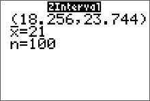
Solution:   \[ \eqalign{ \bar{x} &=\dfrac{(\text{upper confidence limit})+(\text{lower confidence limit})}{2} \cr &=\dfrac{23.744+18.256}{2}\cr & = 21 } \] and \[ \eqalign{ E &=\text{upper confidence limit} - \text{point estimate} \cr &=(\bar{x}+E)-\bar{x}\cr &= 23.744-21\cr & = 2.744 } \]

---

Using the Calculator to find the Confidence Interval

The TI-83/84 Plus calculator can be used to generate confidence intervals for original sample values stored in a list, or you can use the summary statistics $n, \bar{x}$, and $\sigma$. Either enter the data in list L1 or have the summary statistics available, then press the STAT key. Now select TESTS and choose ZInterval. After making the required entries, the calculator display will include the confidence interval in the format of $(\bar{x}-E, \ \ \bar{x}+E)$

---

Finding a z Confidence Interval for the Mean (Statistics)

Example:   A researcher wants to estimate the average amount of time, in hours per day, that a U.S. teenager spends consuming media — watching TV, listening to music, surfing the Web, social networking, and playing video games. A random sample of $n=1000$ U.S. teenagers were polled about the amount of time they spend daily consuming media. The results of the poll produced a mean amount of $7.6$ hours with a standard deviation of 2.2 hours. Use this information to estimate the population mean. Use a 90% level of confidence. (Source: The Washington Post)

1. Press STAT and move the cursor to TESTS.
2. Press 7 for ZInterval.
3. Move the cursor to Stats and press ENTER.
4. Type in the appropriate values.
5. Move the cursor to Calculate and press ENTER.

Calculator Solution:  

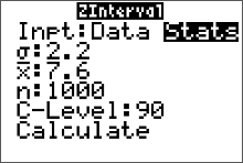
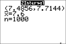
Conclusion:   The 90% confidence interval for $\mu$ is from 7.49 hours to 7.71 hours per day.

---

Finding a z Confidence Interval for the Mean (Data)

Find the 95% confidence interval for the mean using this sample.
45 52 35 22 62 34 42 46 53 58 36 40 43 16 23
54 27 32 24 53 62 67 84 36 44 49 57 35 25 30

1. Enter the data into L1. (Press STAT $\to$ ENTER to access L1)
2. Press STAT and move the cursor to TESTS.
3. Press 7 for ZInterval.
4. Move the cursor to Data and press ENTER.
5. Type in the appropriate values.
6. Move the cursor to Calculate and press ENTER

The population standard deviation $\sigma$ is unknown. Since the sample size is $n \geq30$, you can use the sample standard deviation $s$ as an approximation for $\sigma$. After the data values are entered in L1 (step 1 above), press STAT, move the cursor to CALC, press 1 for 1-Var Stats, then press ENTER. The sample standard deviation of 15.50246551 will be one of the statistics listed. Then continue with step 2. At step 5 on the line for $\sigma$, press VARS for variables, press 5 for Statistics, press 3 for $S_x$.

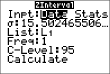
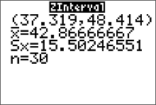
Conclusion:   The 95% confidence interval for $\mu$ is from $37.3$ to $\$48.4$.
Notice the output from ZIinterval command gives us the sample mean and sample standard deviation.

---

Sample Size Determination

As the level of confidence is increased, the confidence interval widens. As the confidence interval widens, the precision of the estimate decreases. One way to improve the precision of an estimate without decreasing the level of confidence is to increase the sample size. But how large a sample size is needed to guarantee a certain level of confidence for a given margin of error? By using the formula for margin of error $$ E = z_c\cdot\frac{\sigma}{\sqrt{n}} $$ a formula can be derived (by solving this formula for $n$) as shown in the next definition.

Example:  A pizza shop owner wishes to find the 95% confidence interval estimate for the true mean cost of a large pepperoni pizza. How large should the sample be if she wishes to be accurate within $\$0.15$? A previous study showed that the standard deviation of the price was $\$0.26$.

Solution:   \[ \eqalign{ n & =\biggr(\frac{z_c\cdot \sigma}{E}\biggr)^2 \cr & =\biggr(\frac{1.96\cdot\$0.26}{\$0.15}\biggr)^2 \cr & = 11.54187378 \color{red}{\text{ always round up!}}\cr & \doteq 12 } \] The minimum sample size required is 12 prices.

---

Try This!!

Question Determine the minimum sample size required when you want to be 99% confident that the sample mean is within two units of the population mean and $\sigma=1.4$. Assume the population is normally distributed.

---

Try This!!

Question A beverage company uses a machine to fill one-liter bottles with water. Assume the population of volumes is normally distributed. The company wants to estimate the mean volume of water the machine is putting in the bottles within one milliliter ($mm$). Determine the minimum sample size required to construct a 96% confidence interval estimate for $\mu$. Assume the population standard deviation is 3 millimeters.

---

Confidence Interval for a Population Proportion $p$

Many research experiments or sample surveys have as their objective the estimation of the proportion of people or objects in a large group that possess a certain, characteristic. Here are some examples:

• The proportion of Americans who have internet access
• The proportion of those who believe there is solid evidence that Earth is getting warmer
• The proportion of residents who closely follow the local news or who often discuss local crime

Each is a practical example of the binomial experiment, and the parameter to be estimated is the binomial proportion, $p$. When the sample size is large, \[ \hat{p}=\frac{x}{n}=\frac{\text{total number of successes}}{\text{total number of trials}} \] is the best point estimator for the population proportion $p$. Since its sampling distribution is approximately normal, with mean $p$ and standard error SE $= \sqrt{\frac{pq}{n}}$,   $\hat{p}$ can be used to construct a confidence interval according to the general approach given here.

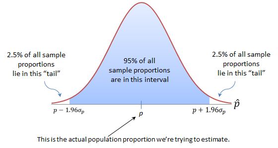
Example:   A reporter wants to estimate the percentage of residents in her city who would rate their city as an excellent place to live. The reporter wants to estimate each percentage by race or ethnicity. It is found that residents in her city are predominantly white, non-hispanic. A random sample of 120 people are selected from among those who categorized their race/ethnicity as "white, non-Hispanic," and 55% indicated they would rate their city as an excellent place to live. Another random sample of 120 "Hispanic" individuals is drawn and suppose 40% indicated they would rate their city as an excellent place to live. Use this information to estimate the population proportion of Hispanic residents who would rate their city as an excellent place to live. Use a 99% level of confidence. (Source: journalism.org)

Solution:   The random variable, $x$ represents the proportion of Hispanic residents among the 120 sampled who would rate their city as an excellent place to live. The point estimate of $p$ is $\hat{p}=0.40$. (There were $x=n\cdot\hat{p}=120\cdot0.40=48$ individual successes.)  Also, notice that both $n\hat{p}>5$ and $n\hat{q}>5$, so that the binomial population distribution we are sampling from is approximately normal. Then, the standard error (the standard deviation of the sampling distribution) can be approximated as \[ \sqrt{\frac{pq}{n}}\approx \sqrt{\frac{\hat{p}\hat{q}}{n}} = \sqrt{\frac{0.40\cdot0.60}{120}}\doteq0.0447213595 \] The value for $z_c$ in the margin of error formula is found with the calculator using $z_c= invnorm\Bigg( \frac{1}{2}(1+c)\Bigg)= invnorm\Bigg( \frac{1}{2}(1+0.99)\Bigg) \doteq 2.58$. The margin of error is then approximated as \[ E= z_{c}\cdot\sqrt{\frac{\hat{p}\hat{q}}{n}}=2.58\cdot0.0447213595\approx0.116 \] The approximate 99% confidence interval is \[ \eqalign{ \hat{p} & \pm \ E\cr 0.40 & \pm \ 0.116\cr } \] Then $0.40-0.116=0.284=28.4\%$ and $0.40+0.116=0.516=51.6\%.$

The 99% confidence interval for $p$ is from 28.4% to 51.6%.

---

Try This!!

A reporter wants to estimate the percentage of U.S. households that have internet. A random sample of 4000 U.S. households found 2880 households that had internet. Construct a 98% confidence interval estimate of the percentage of U.S. households that have internet.

---

Calculator Example

Question     There were 200 nursing applications in a sample, and 12% of the applicants were male. Find the 99% confidence interval for the true proportion of male applicants.

Solution     $x$ is the number of applications by males in $n=200$ applications. We are given the sample proportion, $\hat{p}=12\%$. To get the value of $x$ for the calculator, we use $x=n\cdot\hat{p}=200(0.12) =24$.

1. Press the STAT button on your calculator and move the cursor to TESTS.
2. Press A (ALPHA, MATH) for 1-PropZlnt.
3. Type in the appropriate values.
4. Move the cursor to Calculate and press ENTER.

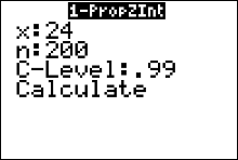
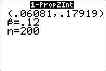
The 99% confidence interval estimate for the population percentage of male applicants is between 6.1% and 17.9%.

---

Sample Size Determination

Example:  You wish to estimate, with 90% confidence, the population proportion of U.S. adults who are confident in the stability of the U.S. banking system. Your estimate must be accurate to within 3% of the population proportion.

1. No preliminary or previous estimate is available. Find the minimum sample size needed.
2. Find the minimum sample size needed, using a prior study that found 43% of U.S. adults are confident in the stability of the system.
3. Compare the results from (a) and (b).

Solution (a):   No preliminary or previous estimate is available for $\hat{p}$ and $\hat{q}=0.50$, so we assume $\hat{p}$ and $\hat{q}=0.50$. We are given $E=3\%=0.03$ and $c=0.90$. Then \[ z_{c}=invnorm\Bigg(\dfrac{1}{2}(1+c)\Bigg)=invnorm\Bigg(\dfrac{1}{2}(1+0.90)\Bigg)\doteq1.64 \] and \[ \eqalign{ n & =\hat{p}\cdot\hat{q}\cdot\biggr(\frac{z_c}{E}\biggr)^2 \cr & ={0.5}\cdot{0.5}\cdot\biggr(\frac{1.64}{0.03}\biggr)^2 \cr & = 747.111111111 \color{red}{\text{ always round up!}}\cr & \doteq 748 } \] The minimum sample size required is 748 U.S. adults.

Solution (b):   A preliminary estimate for $\hat{p}$ was given as 0.43, so the estimate for $\hat{q}=1-\hat{p}=1-0.43=0.57$. We are given $E=3\%=0.03$ and $c=0.90$. Then \[ \eqalign{ n & =\hat{p}\cdot\hat{q}\cdot\biggr(\frac{z_c}{E}\biggr)^2 \cr & ={0.43}\cdot{0.57}\cdot\biggr(\frac{1.64}{0.03}\biggr)^2 \cr & = 732.4677333 \color{red}{\text{ always round up!}}\cr & \doteq 733 } \] The minimum sample size required is 733 U.S. adults.

Solution (c):   Having an estimate of the population proportion reduces the minimum sample size needed.

Try This!!

Question Determine the minimum sample size required when you want to be 95% confident that the sample proportion is within two percentage points of the population proportion. Assume the population is normally distributed.

---

Try This!!

Question A recent report by Pew Research Center estimated that 68% of Americans have smartphones and 45% have tablet computers. How large a sample is needed to estimate the true proportion of Americans with smartphones to within 4% with 86% confidence?

---

Confidence Interval for a Population Mean $\mu$  (small samples)

Suppose you need to estimate the value of $\mu$ but it is impossible or impractical to collect a large sample. Then the estimation procedure outlined above is of no use. This section introduces the estimation procedure that can be used when the sample size is small. Small sample confidence intervals for binomial proportions will be omitted from our discussion.

Student's $t$ Distribution

In discussing the sampling distribution of $\bar{x}$, we made these points:

• When the population distribution is normal, the sampling distribution of $\bar{x}$ and $z = (\bar{x} - \mu)/(\sigma/\sqrt{n})$) both have normal distributions, for any sample size.


• When the original sampled population is not normal, $\bar{x}$,  $z = (\bar{x} - \mu)/(\sigma/\sqrt{n})$, and $z \approx (\bar{x} - \mu)/(s/\sqrt{n})$ all have approximately normal distributions, if the sample size is large $(n\geq30)$.

Unfortunately, when the sample size n is small $(n \text{ less than 30})$, the statistic $(\bar{x} - \mu)/(\sigma/\sqrt{n})$ does not have a normal distribution. Therefore, all the critical values of $z$ that you used before are no longer correct. For example, you cannot say that $\bar{x}$ will lie within 1.96 standard errors of $\mu$   95% of the time. This problem is not new; it was studied by statisticians and experimenters in the early 1900s. To find the sampling distribution of this statistic, there are two ways to proceed:

• Use an empirical approach. Draw repeated samples and compute $(\bar{x} - \mu)/(s/\sqrt{n})$ for each sample. The relative frequency distribution that you construct using these values will approximate the shape and location of the sampling distribution.
• Use a mathematical approach to derive the actual probability density function (the curve that describes the standardized sampling distribution of $\bar{x}$.

The second approach was used by an Englishman named W. S. Gosset in 1908. He derived a complicated formula for the density function of

\[ t=\frac{\bar{x} - \mu}{s/\sqrt{n}} \]

for random samples of size $n$ from a normal population, and he published his results under the pen name ''Student." Ever since, the statistic has been known as Student's $t$. It has the following characteristics:

• The mean, median and mode are all equal to zero.
• The total area under the $t$-distribution curve is 1.
• It is mound-shaped and symmetric about $t = 0$, just like the Standard Normal distribution of $z$.
• It is more variable than $z$ with "heavier tails"; that is, the $t$ curve does not approach the horizontal axis as quickly as $z$ does. This is because the $t$ statistic involves two random quantities, $\bar{x}$ and $s$, whereas the $z$ statistic involves only the sample mean, $\bar{x}$. You can see this phenomenon in the worksheet below.
• The shape of the $t$ distribution depends on the sample size $n$. As $n$ increases, the variability of $t$ decreases because the estimates of $s$ of $\sigma$ is based on more and more information. Eventually, when $n$ is infinitely large, the $t$ and $z$ distributions are identical!

Gosset was a Guinness Brewery employee who needed a distribution that could be used with small samples taken from a normal distributed population. The Irish brewery where he worked did not allow the publication of research results, so Gosset published under the pseudonym "Student."

The divisor $(n - 1)$ in the formula for the sample variance $s^2$ is called the number of degrees of freedom (df) associated with $s^2$.   It determines the shape of the $t$ distribution. The origin of the term degrees of freedom is theoretical and refers to the number of independent squared deviations in $s^2$ that are available for estimating $\sigma^2$.  These degrees of freedom may change for different applications, and since they specify the correct $t$ distribution to use, you need to remember to calculate the correct degrees of freedom for each application.

The table of normal probabilities for the standard normal $z$ distribution is no longer useful in calculating critical values for the margin of error in your confidence interval formula. Instead, you will use the $t$-table (below). The table body lists critical values of $t_{c}$. The first column of the table is a particular number of degrees of freedom. The top row has a percentage area to the left of a vertical line at $t_c$.

Student's $t$ Table

(pdf )

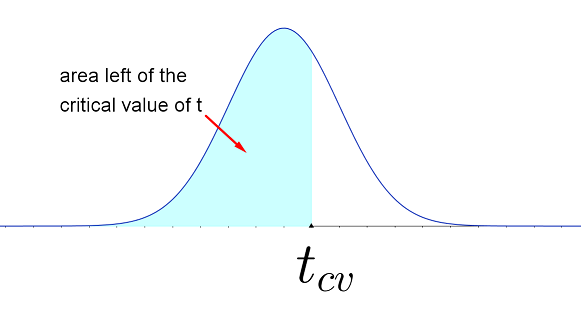
The percentage at the top of the table is equal to the AREA to the LEFT of the critical value, $t_{cv}$, found in the table body.

$$ \begin{array} {r|@{\quad}r@{\,}r@{\,}r@{\,}r@{\,}r@{\,}r@{\,}r@{\,}r@{\,}r@{\,}r@{\,}r} \ \\ df&60.0\%&66.7\%&75.0\%&80.0\%&87.5\%&90.0\%&95.0\%&97.5\%&99.0\%&99.5\% &99.9\% \\ \hline \ \\ 1&0.325&0.577&1.000&1.376&2.414&3.078&6.314&12.706&31.821&63.657&318.31 \\ 2&0.289&0.500&0.816&1.061&1.604&1.886&2.920&4.303&6.965&9.925&22.327 \\ 3&0.277&0.476&0.765&0.978&1.423&1.638&2.353&3.182&4.541&5.841&10.215 \\ 4&0.271&{0.464}&0.741&0.941&1.344&1.533&2.132&2.776&3.747&\color{red}{4.604}&7.173 \\ 5&0.267&0.457&0.727&0.920&1.301&1.476&2.015&2.571&3.365&4.032&5.893 \\ 6&0.265&0.453&0.718&0.906&1.273&1.440&1.943&2.447&3.143&3.707&5.208 \\ 7&0.263&0.449&\color{red}{0.711}&0.896&1.254&1.415&1.895&2.365&2.998&3.499&4.785 \\ 8&0.262&0.447&0.706&0.889&1.240&1.397&1.860&2.306&2.896&3.355&4.501 \\ 9&0.261&0.445&0.703&0.883&1.230&1.383&1.833&2.262&2.821&3.250&4.297 \\ 10&0.260&0.444&0.700&0.879&1.221&\color{red}{1.372}&1.812&2.228&2.764&3.169&4.144 \\ 11&0.260&0.443&0.697&0.876&1.214&1.363&1.796&2.201&2.718&3.106&4.025 \\ 12&0.259&0.442&0.695&0.873&1.209&1.356&1.782&2.179&2.681&3.055&3.930 \\ 13&0.259&0.441&0.694&0.870&1.204&1.350&1.771&2.160&2.650&3.012&3.852 \\ 14&0.258&0.440&0.692&0.868&1.200&1.345&1.761&\color{red}{2.145}&2.624&2.977&3.787 \\ 15&0.258&0.439&0.691&0.866&1.197&1.341&1.753&2.131&2.602&2.947&3.733 \\ 16&0.258&0.439&0.690&0.865&1.194&1.337&1.746&2.120&2.583&2.921&3.686 \\ 17&0.257&0.438&0.689&0.863&1.191&1.333&1.740&2.110&2.567&2.898&3.646 \\ 18&0.257&0.438&0.688&0.862&1.189&1.330&1.734&2.101&2.552&2.878&3.610 \\ 19&0.257&0.438&0.688&0.861&1.187&1.328&1.729&2.093&2.539&2.861&3.579 \\ 20&0.257&0.437&0.687&0.860&1.185&1.325&1.725&2.086&2.528&2.845&3.552 \\ 21&0.257&0.437&0.686&0.859&1.183&1.323&1.721&2.080&2.518&2.831&3.527 \\ 22&0.256&0.437&0.686&0.858&1.182&1.321&\color{red}{1.717}&2.074&2.508&2.819&3.505 \\ 23&0.256&0.436&0.685&0.858&1.180&1.319&1.714&2.069&2.500&2.807&3.485 \\ 24&0.256&0.436&0.685&0.857&1.179&1.318&1.711&2.064&2.492&2.797&3.467 \\ 25&0.256&0.436&0.684&0.856&1.178&1.316&1.708&2.060&2.485&2.787&3.450 \\ 26&0.256&0.436&0.684&0.856&1.177&1.315&1.706&2.056&2.479&2.779&3.435 \\ 27&0.256&0.435&0.684&0.855&1.176&1.314&1.703&2.052&2.473&2.771&3.421 \\ 28&0.256&0.435&0.683&0.855&1.175&1.313&1.701&2.048&2.467&2.763&3.408 \\ 29&0.256&0.435&0.683&0.854&1.174&1.311&1.699&2.045&2.462&2.756&3.396 \\ 30&0.256&0.435&0.683&0.854&1.173&1.310&1.697&2.042&2.457&2.750&3.385 \\ 35&0.255&0.434&0.682&0.852&1.170&1.306&1.690&2.030&2.438&2.724&3.340 \\ 40&0.255&0.434&0.681&0.851&1.167&1.303&1.684&2.021&2.423&2.704&3.307 \\ 45&0.255&0.434&0.680&0.850&1.165&1.301&1.679&2.014&2.412&2.690&3.281 \\ 50&0.255&0.433&0.679&0.849&1.164&1.299&1.676&2.009&2.403&2.678&3.261 \\ 55&0.255&0.433&0.679&0.848&1.163&1.297&1.673&2.004&2.396&2.668&3.245 \\ 60&0.254&0.433&0.679&0.848&1.162&1.296&1.671&2.000&2.390&2.660&3.232 \\ \infty &0.253&0.431&0.674&0.842&1.150&1.282&1.645&1.960&2.326&2.576&3.090 \end{array} $$

---

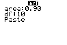
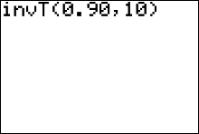
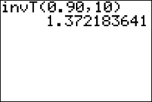
Example 1:   For a $t$ distribution with 10 degrees of freedom, the value of $t$ that has an area 0.90 to its left is found in row 10 in the column marked "90%." You should verify that this is $\color{red}{t=1.372}$

---

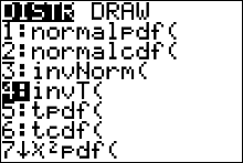
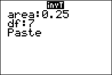
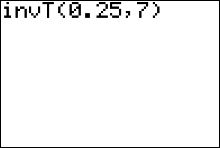
Alternatively, you can find this critical value of $t$ using the $\color{red}{invT}$ (the t inverse) function on the TI83/84+ calculator:

1. Press 2nd then vars.
2. Select the invT function by pressing 4
3. Insert values for area and degrees of freedom, $df$ (where $df=n-1$).
   Note that the calculator expects you to input an area left of the unknown value of $t$.
4. Highlight the word "paste" then press enter. This pastes the command "invT(area, df)" over to the home screen.
5. After the command is pasted, press enter again

---

Example 2:   Find the $t$ value that represents the $t$-score in the 50th percentile.

Solution:   That value of $t$ will be 0 for any sample size, since every $t$ distribution curve is centered at the origin.

---

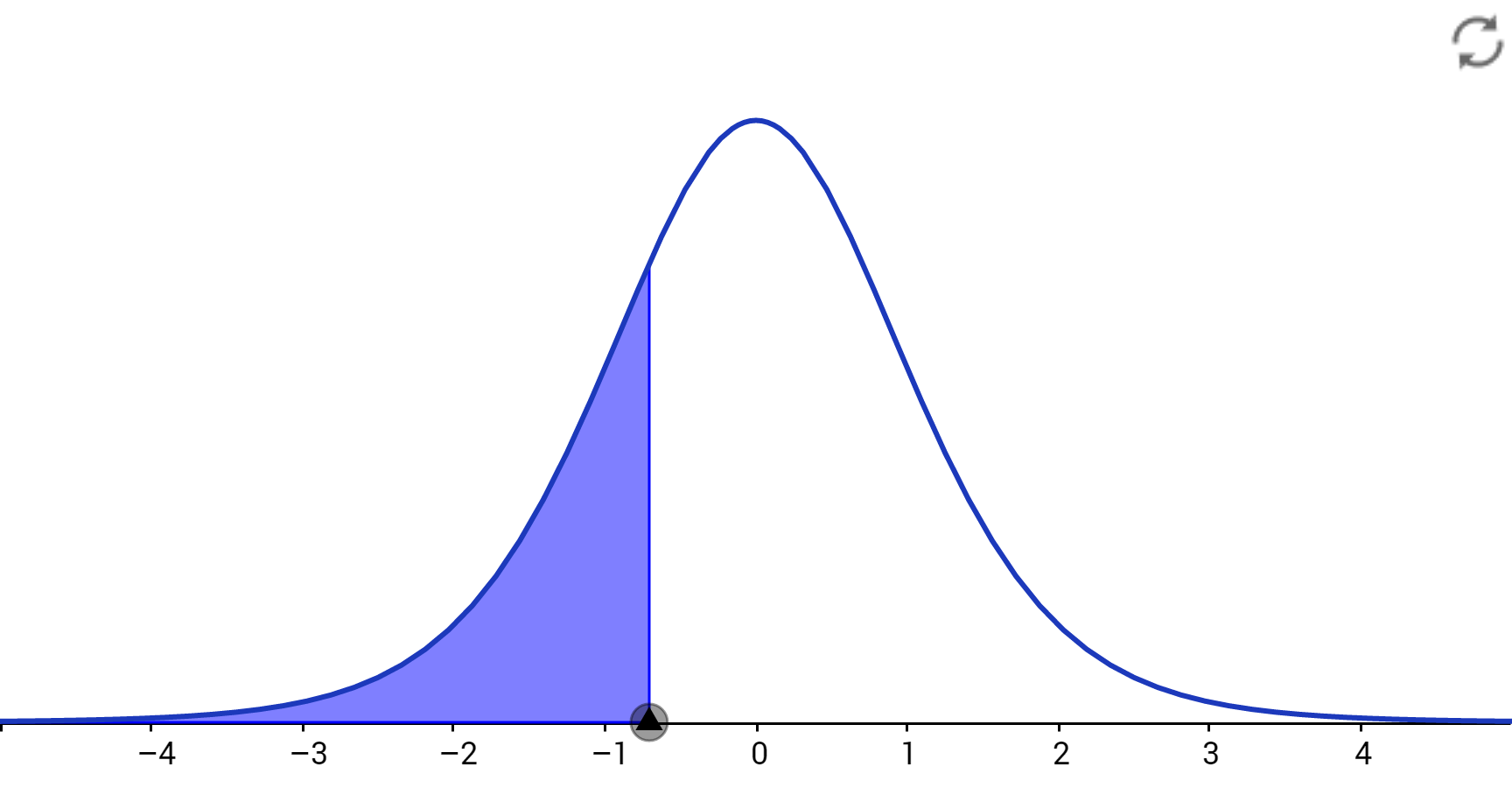
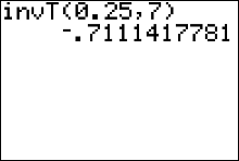
Example 3:   Find the $t$ value that represents the first quartile of $t$-scores. Assume $n=8.$

Solution:   The degrees of freedom that specify the correct $t$ distribution are $df = n - 1 = 7$; so, the critical value is in the 7th row of the table. The $t$ value that represents the first quartile of $t$-scores is the value separating the lower 25% of $t$-scores from the upper 75%. The $t$-value we are looking for must be in the lower portion of the distribution, with area 25% to its left, as shown in the figure below. Since the $t$ distribution is symmetric about 0, this value is simply the negative (opposite) of the $t$-value that has an area of 0.75 to its left, or $\color{red}{-t = -0.711}$. Notice the table won't give you negative values, instead we have to find the $t$-value that has an area of 1-0.25 = 0.75 to its left and find it's opposite.

---

Alternatively, you can find this critical value of $t$ using the $\color{red}{invT}$ (the t inverse) function on the TI83/84+ calculator:

1. Press 2nd then vars.
2. Select the invT function by pressing 4
3. Insert values for area and degrees of freedom, $df$ (where $df=n-1$).
   Note that the calculator expects you to input an area left of the unknown value of $t$
4. Highlight the word "paste" then press enter. This pastes the command "invT(area, df)" over to the home screen.
5. After the command is pasted, press enter again

---

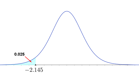
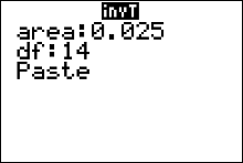
Example 4:   Suppose you have a sample of size 15 from a normal distribution. Find a value of $t$ such that only 2.5% of all values of $t$ will be smaller.

Solution:   The degrees of freedom that specify the correct $t$ distribution are $df = n - 1 = 14$, and the necessary $t$-value must be in the lower portion of the distribution, with area 2.5% to its left, as shown in the figure below. Since the $t$ distribution is symmetric about 0, this value is simply the negative of the value on the right-hand side with area 0.975 to its left, or $-t = \color{red}{-2.145}$.

---

Values of $t$ given in the $t$-table are output values from Gosset's complicated formula that produces the standardized sampling distribution curve. These values have been rounded three decimal place value columns (to the thousandths).

---

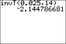
Example 6:   Find the value of $t_c$ needed to set up a 90% percent confidence interval estimate for $\mu$. Assume the sample size is 23.

Solution:   The degrees of freedom that specify the correct $t$ distribution are $df = n - 1 = 23 - 1 =22.$ The area under the standardized sampling distribution of $t$-scores just left of a vertical line at $t_c$ is $\frac{1}{2}(1-c)+c$; or equivalently, $\frac{1}{2}(1+c) = \frac{1}{2}(1+0.90) = 0.95$. Therefore, the value of $t$ we need can be found in row 22 of the table, in the column labeled "95%." This value is $\color{red}{1.717}$

---

Alternatively, you can find this critical value of $t$ using the $\color{red}{invT}$ (the t inverse) function on the TI83/84+ calculator:

1. Press 2nd then vars.
2. Select the invT function by pressing 4
3. Insert values for area and degrees of freedom, $df$ (where $df=n-1$).
   Note that the calculator expects you to input the value given by the formula $\frac{1}{2}(1+c)$ for area.
4. Highlight the word "paste" then press enter. This pastes the command "invT(area, df)" over to the home screen.
5. After the command is pasted, press enter again

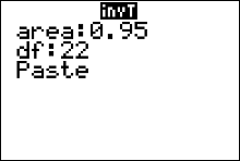
A common mistake for those using the invT function on the calculator is that they input the confidence level, $c$, for the area instead of inputting $\frac{1}{2}(1+c)$ for area. Try to avoid this mistake.

---

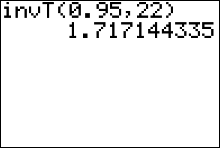
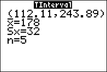
Example:  Suppose that for a random sample of 5 computers at a certain electronics store, the mean repair cost was $\$178$. The sample standard deviation was $\$32$. Assume the population is normally distributed. Construct a 99% confidence interval estimate for the population mean repair cost.

Solution:   The point estimate for $\mu$ is the sample mean $\bar{x}=\$178$. The number of degrees of freedom is $df=n-1=4$, which tells us our critical value, $t_{c}$ for the margin of error formula is located on the 4th row of the table. This critical value has an area left equal to 99.5% since \[ \eqalign{ \frac{1}{2}(1+c) & =\frac{1}{2}(1+0.99)\cr & = 0.995\cr & = 99.5\% } \] The area left of the critical value is then 99.5%, with 4 degrees of freedom. This give us the value $t=4.604$ from the $t$-table. The margin of error is

\[ E=t_{c}\cdot\frac{s}{\sqrt{n}} =4.604\cdot \frac{\$32}{\sqrt{5}} \approx \$65.89 \] and the approximate 99% confidence interval is

$\bar{x}-E$   <  $\mu$  <  $\bar{x}+E$

$\$178-\$65.89$   <  $\mu$  <  $\$178+\$65.89$

$\$112.11$   <  $\mu$  <  $\$243.89$

We are 99% confidence that the interval from $\$112.11$ to $\$243.89$ contains the true value of the population mean repair cost, $\mu$.

---

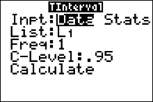
Using the Calculator to find the Confidence Interval

The TI-83/84 Plus calculator can be used to generate confidence intervals for original sample values stored in a list, or you can use the summary statistics $n, \bar{x}$, and $s$. Either enter the data in list L1 or have the summary statistics available, then press the STAT key. Now select TESTS and choose TInterval. After making the required entries, the calculator display will include the confidence interval in the format of $(\bar{x}-E, \ \ \bar{x}+E)$

---

Finding a $t$ Confidence Interval for the Mean (Statistics)

Example:  Suppose that for a random sample of 5 computers at a certain electronics store, the mean repair cost was $\$178$. The sample standard deviation was $\$32$. Assume the population is normally distributed. Construct a 99% confidence interval estimate for the population mean repair cost.

1. Press STAT and move the cursor to TESTS.
2. Press 8 for TInterval.
3. Move the cursor to Stats and press ENTER.
4. Type in the appropriate values.
5. Move the cursor to Calculate and press ENTER.

Calculator Solution:  

Conclusion:   The 99% confidence interval for $\mu$ is from $\$112.11$ to $\$243.89$.

---

Finding a $t$ Confidence Interval for the Mean (Data)

Find the 95% confidence interval for the mean using this sample.
625   675   535   406   512   680   483   522   619   575

1. Enter the data into L1. (Press STAT $\to$ ENTER to access L1)
2. Press STAT and move the cursor to TESTS.
3. Press 8 for TInterval.
4. Move the cursor to Data and press ENTER.
5. Type in the appropriate values.
6. Move the cursor to Calculate and press ENTER

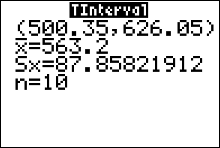
Conclusion:   The 95% confidence interval for $\mu$ is from 500.35 to 626.05.
Notice the output from the TInterval command also gives us the point estimate (the mean of the sample), and the sample standard deviation, $s$.

---

Comparing the $t$ and $z$ Distributions

Look at one of the columns in the $t$-table. As the degrees of freedom increase, the critical value of $t$ decreases until, when $df = \infty$; the critical $t$-value is the same as the critical $z$-value for the same tail area. For example, when the area right of $t$ is 95%, the values of $t_{c}$ start at 6.314 for 1 degree of freedom and decrease to a minimum of $t_{c} = z_{c} = 1.645$. This helps to explain why we use $n = 30$ as the somewhat arbitrary dividing line between large and small samples. When $n = 30 \quad (df = 29)$, the critical values of $t$ are quite close to their normal counterparts. Notice that $t_{c} = 1.699$ is quite close to $z_{c} = 1.645$. Rather than produce a $t$ table with rows for many more degrees of freedom, the critical values of $z$ are sufficient when the sample size reaches $n = 30$.

Assumptions Behind Student's t Distribution

The critical values in the $t$-table will allow you to make reliable inferences only if you follow all the rules; that is, your sample must meet these requirements specified by the $t$ distribution:

• The sample must be randomly selected.
• The population from which you are sampling must be normally distributed.

These requirements may seem quite restrictive. How can you possibly know the shape of the probability distribution for the entire population if you have only a sample? If this were a serious problem, however, the $t$ statistic could be used in only very limited situations. Fortunately, the shape of the $t$ distribution is not affected very much as long as the sampled population has an approximately mound­shaped distribution. Statisticians say that the $t$ statistic is robust, meaning that the distribution of the statistic does not change significantly when the normality assumptions are violated.

How can you tell whether your sample is from a normal population? Although there are statistical procedures designed for this purpose. the easiest and quickest way to check for normality is to use the graphical techniques of earlier chapters: Draw a dotplot or construct a stem and leaf plot. As long as your plot tends to "mound up" in the center, you can be fairly safe in using the $t$ statistic for making inferences.

The random sampling requirement, on the other hand, is quite critical if you want to produce reliable inferences. If the sample is not random, or if it does not at least behave as a random sample, then your sample results may be affected by some unknown factor and your conclusions may be incorrect. When you design an experiment or read about experiments conducted by others, look critically at the way the data have been collected!

---

Many textbooks title this section setting up a Confidence Interval for a Population Mean $\mu$  (with $\sigma$ unknown/not given). However,

• if $\sigma$ is unknown and $n\geq30$, the sampling distribution of $\bar{x}$ will be bell-shaped-- no matter what the shape of the population distribution is -- and the distribution of $z$ scores of all the sample means in the sampling distribution can be approximated with the Standard Normal distribution, even if we use the sample standard deviation, $s$ in place of the unknown population standard deviation, $\sigma$.
• On the other hand, if the population distribution is not normal and $n$ is less than 30 then we cannot use the standard normal distribution or $t$ distribution.

---

Confidence Intervals for the Population Variance, \(\sigma^2\), and Standard Deviation, \(\sigma\)

Sometimes the population variance, \(\sigma^2\), is the primary objective in an experimental investigation. In the manufacturing process, it is necessary to control the amount that a process varies. Consider these examples

• In the manufacture of medicines the variance and standard deviation of the medication in pills plays an important role in making sure patients receive the proper dosage.
• Machined parts in a manufacturing process must be produced with the minimum variability in order to reduce out-of-size, or defective parts. For instance, when products that fit together (such as pipes) are manufactured, it is important to keep the variations of the diameters of the products as small as possible.
• Scientific measuring instruments must provide unbiased readings with a very small error of measurement. An aircraft altimeter that measures correct altitude on the average is fairly useless if measurements are in error by as much as 1000 feet above or below the correct altitude.
• Aptitude tests must be designed so that scores will exhibit a reasonable amount of variability. For example, an 800-point test is not very discriminatory if all students score between 601 and 605

How can you measure, and consequently control, the amount of variation in parts? You can start by finding a point estimate.

Then you can use a chi-square distribution to construct a confidence interval for the variance and standard deviation.

The Chi-Square $(\chi^2)$ Distribution

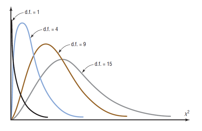
The chi-square variable is similar to the $t$ variable in that its distribution is a family of curves based on the number of degrees of freedom. The shape of a specific chi-square distribution depends on the number of degrees of freedom. The symbol for chi-square is $\chi^2$ (Greek letter chi, pronounced “ki”). Several of the distributions are shown in the figure above, along with the corresponding degrees of freedom. The chi-square distribution is obtained from the values of $(n-1)s^2/\sigma^2$ when random samples are selected from a normally distributed population whose variance is $\sigma^2$.

The Chi-Square $(\chi^2)$ Table

(LINK TO PDF COPY OF TABLE)

The percentage at the top of the table is equal to the AREA to the LEFT of $\chi^2$; where $\chi^2$ is located both along the horizontal axis and in the table body.

$$ \begin{array} {r|@{\ }r@{\ }r@{\ }r@{\ }r@{\ }r@{\ }r@{\ }}\\ \ \\ df&0.1\%&0.5\%&1.0\%&2.5\%&5.0\%&10.0\%&12.5\%&20.0\%&25.0\%&33.3\%&50.0\%\\ \hline \ \\ 1&0.000&0.000&0.000&0.001&0.004&0.016&0.025&0.064&0.102&0.186&0.455\\ 2&0.002&0.010&0.020&0.051&0.103&0.211&0.267&0.446&0.575&0.811&1.386\\ 3&0.024&0.072&0.115&0.216&0.352&0.584&0.692&1.005&1.213&1.568&2.366\\ 4&0.091&0.207&0.297&0.484&0.711&1.064&1.219&1.649&1.923&2.378&3.357\\ 5&0.210&0.412&0.554&0.831&1.145&1.610&1.808&2.343&2.675&3.216&4.351\\ 6&0.381&0.676&0.872&1.237&1.635&2.204&2.441&3.070&3.455&4.074&5.348\\ 7&0.598&0.989&1.239&1.690&2.167&2.833&3.106&3.822&4.255&4.945&6.346\\ 8&0.857&1.344&1.646&2.180&2.733&3.490&3.797&4.594&5.071&5.826&7.344\\ 9&1.152&1.735&2.088&2.700&3.325&4.168&4.507&5.380&5.899&6.716&8.343\\ 10&1.479&2.156&2.558&3.247&3.940&4.865&5.234&6.179&6.737&7.612&9.342\\ 11&1.834&2.603&3.053&3.816&4.575&5.578&5.975&6.989&7.584&8.514&10.341\\ 12&2.214&3.074&3.571&4.404&5.226&6.304&6.729&7.807&8.438&9.420&11.340\\ 13&2.617&3.565&4.107&5.009&5.892&7.042&7.493&8.634&9.299&10.331&12.340\\ 14&3.041&4.075&4.660&5.629&6.571&7.790&8.266&9.467&10.165&11.245&13.339\\ 15&3.483&4.601&5.229&6.262&7.261&8.547&9.048&10.307&11.037&12.163&14.339\\ 16&3.942&5.142&5.812&6.908&7.962&9.312&9.837&11.152&11.912&13.083&15.338\\ 17&4.416&5.697&6.408&7.564&8.672&10.085&10.633&12.002&12.792&14.006&16.338\\ 18&4.905&6.265&7.015&8.231&9.390&10.865&11.435&12.857&13.675&14.931&17.338\\ 19&5.407&6.844&7.633&8.907&10.117&11.651&12.242&13.716&14.562&15.859&18.338\\ 20&5.921&7.434&8.260&9.591&10.851&12.443&13.055&14.578&15.452&16.788&19.337\\ 21&6.447&8.034&8.897&10.283&11.591&13.240&13.873&15.445&16.344&17.720&20.337\\ 22&6.983&8.643&9.542&10.982&12.338&14.041&14.695&16.314&17.240&18.653&21.337\\ 23&7.529&9.260&10.196&11.689&13.091&14.848&15.521&17.187&18.137&19.587&22.337\\ 24&8.085&9.886&10.856&12.401&13.848&15.659&16.351&18.062&19.037&20.523&23.337\\ 25&8.649&10.520&11.524&13.120&14.611&16.473&17.184&18.940&19.939&21.461&24.337\\ 26&9.222&11.160&12.198&13.844&15.379&17.292&18.021&19.820&20.843&22.399&25.336\\ 27&9.803&11.808&12.879&14.573&16.151&18.114&18.861&20.703&21.749&23.339&26.336\\ 28&10.391&12.461&13.565&15.308&16.928&18.939&19.704&21.588&22.657&24.280 &27.336\\ 29&10.986&13.121&14.256&16.047&17.708&19.768&20.550&22.475&23.567&25.222 &28.336\\ 30&11.588&13.787&14.953&16.791&18.493&20.599&21.399&23.364&24.478&26.165 &29.336\\ 35&14.688&17.192&18.509&20.569&22.465&24.797&25.678&27.836&29.054&30.894 &34.336\\ 40&17.916&20.707&22.164&24.433&26.509&29.051&30.008&32.345&33.660&35.643 &39.335\\ 45&21.251&24.311&25.901&28.366&30.612&33.350&34.379&36.884&38.291&40.407 &44.335\\ 50&24.674&27.991&29.707&32.357&34.764&37.689&38.785&41.449&42.942&45.184 &49.335\\ 55&28.173&31.735&33.570&36.398&38.958&42.060&43.220&46.036&47.610&49.972 &54.335\\ 60&31.738&35.534&37.485&40.482&43.188&46.459&47.680&50.641&52.294&54.770 &59.335 \end{array} $$



$$ \begin{array} {r|@{\ }r@{\ }r@{\ }r@{\ }r@{\ }r@{\ }r@{\ }r@{\ }r@{\ }r@{\ }r@{\ }r} \ \\ df&60.0\%&66.7\%&75.0\%&80.0\%&87.5\%&90.0\%&95.0\%&97.5\%&99.0\%&99.5\% &99.9\%\\ \hline \ \\ 1&0.708&0.936&1.323&1.642&2.354&2.706&3.841&5.024&6.635&7.879&10.828\\ 2&1.833&2.197&2.773&3.219&4.159&4.605&5.991&7.378&9.210&10.597&13.816\\ 3&2.946&3.405&4.108&4.642&5.739&6.251&7.815&9.348&11.345&12.838&16.266\\ 4&4.045&4.579&5.385&5.989&7.214&7.779&9.488&11.143&13.277&14.860&18.467\\ 5&5.132&5.730&6.626&7.289&8.625&9.236&11.070&12.833&15.086&16.750&20.515\\ 6&6.211&6.867&7.841&8.558&9.992&10.645&12.592&14.449&16.812&18.548&22.458\\ 7&7.283&7.992&9.037&9.803&11.326&12.017&14.067&16.013&18.475&20.278&24.322\\ 8&8.351&9.107&10.219&11.030&12.636&13.362&15.507&17.535&20.090&21.955&26.125\\ 9&9.414&10.215&11.389&12.242&13.926&14.684&16.919&19.023&21.666&23.589 &27.877\\ 10&10.473&11.317&12.549&13.442&15.198&15.987&18.307&20.483&23.209&25.188 &29.588\\ 11&11.530&12.414&13.701&14.631&16.457&17.275&19.675&21.920&24.725&26.757 &31.264\\ 12&12.584&13.506&14.845&15.812&17.703&18.549&21.026&23.337&26.217&28.300 &32.910\\ 13&13.636&14.595&15.984&16.985&18.939&19.812&22.362&24.736&27.688&29.819 &34.528\\ 14&14.685&15.680&17.117&18.151&20.166&21.064&23.685&26.119&29.141&31.319 &36.123\\ 15&15.733&16.761&18.245&19.311&21.384&22.307&24.996&27.488&30.578&32.801 &37.697\\ 16&16.780&17.840&19.369&20.465&22.595&23.542&26.296&28.845&32.000&34.267 &39.252\\ 17&17.824&18.917&20.489&21.615&23.799&24.769&27.587&30.191&33.409&35.718 &40.790\\ 18&18.868&19.991&21.605&22.760&24.997&25.989&28.869&31.526&34.805&37.156 &42.312\\ 19&19.910&21.063&22.718&23.900&26.189&27.204&30.144&32.852&36.191&38.582 &43.820\\ 20&20.951&22.133&23.828&25.038&27.376&28.412&31.410&34.170&37.566&39.997 &45.315\\ 21&21.991&23.201&24.935&26.171&28.559&29.615&32.671&35.479&38.932&41.401 &46.797\\ 22&23.031&24.268&26.039&27.301&29.737&30.813&33.924&36.781&40.289&42.796 &48.268\\ 23&24.069&25.333&27.141&28.429&30.911&32.007&35.172&38.076&41.638&44.181 &49.728\\ 24&25.106&26.397&28.241&29.553&32.081&33.196&36.415&39.364&42.980&45.559 &51.179\\ 25&26.143&27.459&29.339&30.675&33.247&34.382&37.652&40.646&44.314&46.928 &52.620\\ 26&27.179&28.520&30.435&31.795&34.410&35.563&38.885&41.923&45.642&48.290 &54.052\\ 27&28.214&29.580&31.528&32.912&35.570&36.741&40.113&43.195&46.963&49.645 &55.476\\ 28&29.249&30.639&32.620&34.027&36.727&37.916&41.337&44.461&48.278&50.993 &56.892\\ 29&30.283&31.697&33.711&35.139&37.881&39.087&42.557&45.722&49.588&52.336 &58.301\\ 30&31.316&32.754&34.800&36.250&39.033&40.256&43.773&46.979&50.892&53.672 &59.703\\ 35&36.475&38.024&40.223&41.778&44.753&46.059&49.802&53.203&57.342&60.275 &66.619\\ 40&41.622&43.275&45.616&47.269&50.424&51.805&55.758&59.342&63.691&66.766 &73.402\\ 45&46.761&48.510&50.985&52.729&56.052&57.505&61.656&65.410&69.957&73.166 &80.077\\ 50&51.892&53.733&56.334&58.164&61.647&63.167&67.505&71.420&76.154&79.490 &86.661\\ 55&57.016&58.945&61.665&63.577&67.211&68.796&73.311&77.380&82.292&85.749 &93.168\\ 60&62.135&64.147&66.981&68.972&72.751&74.397&79.082&83.298&88.379&91.952 &99.607 \end{array} $$

Finding Critical Values of $\chi^2$

There are two values of chi, called critical values, that we need to find before we can set up a confidence interval estimate for the population variance and standard deviation. The notation that we use for the two critical values is $\chi^2_L$ and $\chi^2_R$. The calculator doesn't easily help us obtain these values. So we use the chi-square table to lookup the two critical values.

To find the critical value $\chi^2$ on the table we need two things

1. degrees of freedom given by the formula $df = n-1$
2. the area to the LEFT of the critical value

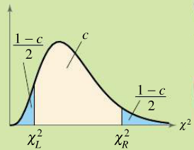
Example:   Find the critical values $\chi^2_L$ and $\chi^2_R$ needed to set up a 95% confidence interval when the sample size is 18.

Solution:   Because the sample size is 18, $$ df =n-1=17$$ The areas to the left of $\chi^2_L$ and $\chi^2_R$ are

Area to the left of $\chi^2_L = \dfrac{1-c}{2}=\dfrac{1-.95}{2}=0.025=2.5\%$



Area to the left of $\chi^2_R = \dfrac{1+c}{2}=\dfrac{1+.95}{2}=0.975=97.5\%$

Using $df=17$ and the areas 2.5% and 97.5% you can find the critical values off of the chi-square table. We find that $$\chi^2_L =7.564$$ and $$\chi^2_R =30.191$$ So, for a chi-square distribution curve with 17 degrees of freedom, 95% of the area under the curve lies between 7.564 and 30.191.

---

Try This!!

Question Find the critical values $\chi^2_L$ and $\chi^2_R$ needed to set up a 90% confidence interval when the sample size is 11.

Example:   You randomly select and weigh a sample of 30 allergy medicine pills. The sample standard deviation is 1.2 milligrams. Assuming the weights are normally distributed, construct 99% confidence intervals for the population variance and standard deviation.

Solution:   Because the sample size is 30, $$ df =n-1=29$$ The areas to the left of $\chi^2_L$ and $\chi^2_R$ are

Area to the left of $\chi^2_L = \dfrac{1-c}{2}=\dfrac{1-.99}{2}=0.005=0.5\%$



Area to the left of $\chi^2_R = \dfrac{1+c}{2}=\dfrac{1+.99}{2}=0.995=99.5\%$

Using $df=29$ and the areas 0.5% and 99.5% you can find the critical values off of the chi-square table. We find that $$\chi^2_L =13.121$$ and $$\chi^2_R =52.336$$

The left endpoint of the confidence interval is $$ \dfrac{(n-1)s^2}{\chi^2_R}=\dfrac{(30-1)1.2^2}{52.336}=0.80 $$

The right endpoint of the confidence interval is $$ \dfrac{(n-1)s^2}{\chi^2_L}=\dfrac{(30-1)1.2^2}{13.121}=3.18 $$

The confidence interval for $\sigma^2$ is $$ \dfrac{(n-1)s^2}{\chi^2_R} < \sigma^2 < \dfrac{(n-1)s^2}{\chi^2_L} $$ or $$0.80 < \sigma^2 < 3.18$$

The confidence interval formula for $\sigma$ is $$ \sqrt{\dfrac{(n-1)s^2}{\chi^2_R}} < \sigma < \sqrt{\dfrac{(n-1)s^2}{\chi^2_L}} $$ or equivalently, $$ \sqrt{\dfrac{(30-1)1.2^2}{52.336}} < \sigma < \sqrt{\dfrac{(30-1)1.2^2}{13.121}} $$ or $$ 0.89 < \sigma < 1.78 $$ With 99% confidence, you can say that the population variance is between 0.80 milligrams squared and 3.18 milligrams squared, and the population standard deviation is between 0.89 milligrams and 1.78 milligrams.

---

Try This!!

Question Find the 95% confidence intervals for the population variance and standard deviation of the medicine weights.