Section 15.1: Goodness of Fit Test

Goodness of Fit Test

In addition to being used to test a single variance, the chi-square statistic can be used to see whether a frequency distribution fits a specific pattern. When you are testing to see whether a frequency distribution fits a specific pattern, you can use the chi-square goodness-of-fit test.

For example, a craft brewery wants to see if consumers have any preference among four new flavors of beer. A sample of opinions from 100 people provided these data: $$ \begin{array}{c|c|c|c} Red \ Pill & Crackalicious & Bavarian & Stumbling \ Cletus \\ Brew & Schwartzbier & Dankenweizen & Amber \ Ale \\ \hline 22 & 28 & 20 & 30\\ \end{array} $$



If there were no preference, you would expect each flavor of beer to be selected with equal frequency, or with a 25% frequency. That is, approximately 25 people in the sample would have selected each flavor of craft beer, had there been no preference.

Since the frequencies for each flavor were obtained from a sample, these actual frequencies are called the observed frequencies. The frequencies obtained by calculation (as if there were no preference) are called the expected frequencies. A completed table for the test is shown.
$$ \begin{array}{c|c|c|c|c} & Red \ Pill & Crackalicious & Bavarian & Stumbling \ Cletus \\ & Brew & Schwartzbier & Dankenweizen & Amber \ Ale \\ \hline Observed & 22 & 28 & 20 & 30\\ \\ \hline Expected & 25 & 25 & 25 & 25\\ \end{array} $$ The observed frequencies will almost always differ from the expected frequencies due to sampling error; that is, the values differ from sample to sample. But the question is: Are these differences significant (a preference exists), or are they due to chance? The chi-square goodness-of-fit test will enable the researcher to determine the answer. Before computing the test value, you must state the hypotheses. The null hypothesis should be a statement indicating that there is no difference or no change. For this example, the hypotheses are as follows: \[ \eqalign{ H_0: \quad & \text{Consumers show no preference for any of the flavor} \cr H_a: \quad & \text{Consumers show a preference} } \] Another way equivalent way to define the hypotheses is define the following population proportions: \[ \eqalign{ p_1 = & \text{the proportion of brewery customers who prefer Red Pill Brew} \cr p_2 = & \text{the proportion of brewery customers who prefer the Crackalicious Brew} \cr p_3 = & \text{the proportion of brewery customers who prefer Bav. Dankenweizen Brew} \cr p_4 = & \text{the proportion of brewery customers who prefer Stumbling Cletus Brew} } \] Then the hypotheses are as follows: \[ \eqalign{ H_0: \quad & p_1 =p_2 =p_3 =p_4 =0.25 \cr H_a: \quad & \text{at least one of the population proportions is not 0.25} } \]

Example 1

Is there enough evidence to reject the claim that there is no preference in the selection of craft beers using the sample data given below? Use $\alpha=0.05.$

$$ \begin{array}{c|c|c|c} Red \ Pill & Crackalicious & Bavarian & Stumbling \ Cletus \\ Brew & Schwartzbier & Dankenweizen & Amber \ Ale \\ \hline \color{red}{22} & \color{green}{28} & \color{blue}{20} & \color{orange}{30}\\ \end{array} $$

Solution

Step 1    State the null and alternative hypothesis. \[ \eqalign{ H_0: \quad & \text{Consumers show no preference for any of the flavor} \cr H_a: \quad & \text{Consumers show a preference} } \] or that \[ \eqalign{ H_0: \quad & p_1 =p_2 =p_3 =p_4 =0.25 \cr H_a: \quad & \text{at least one of the population proportions is not 0.25} } \] Step 2    Find the value of your test statistic with the Chi-Square with the formula $\qquad\chi^2=\displaystyle\sum\frac{(O-E)^2}{E}$ \[ \eqalign{ \chi^2 & = \sum\frac{(O-E)^2}{E} \cr\cr & = \frac{( \color{red}{22}-25)^2}{25}+ \frac{(\color{green}{28}-25)^2}{25}+ \frac{(\color{blue}{20}-25)^2}{25}+ \frac{(\color{orange}{30}-25)^2}{25} \cr\cr & = 2.72 } \] Step 3    Draw a picture of the Chi-Square Distribution (centered at df=number of categories minus1), and mark the location of your test statistic value along the x-axis in the right tail of your graph.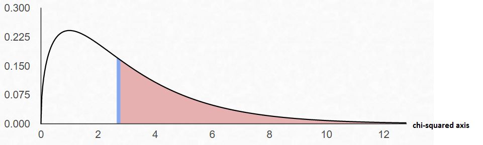

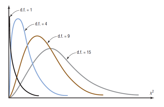
In the goodness-of-fit test, the degrees of freedom are equal to the number of categories minus 1. For this example, there are four categories (4 different flavors of beer); hence, the degrees of freedom are $4-1=3$. This is so because the number of subjects in each of the first three categories is free to vary. But in order for the sum to be 100 -- the total number of subjects -- the number of subjects in the last category is fixed.

Step 4    Find the p-value. This will always be the area to the right of your test statistic. Find this value with your calculator's $\chi^2 \ cdf$ command. Use \[ \eqalign{ p-val & = \chi^2 \ cdf(\text{test stat value}, 10^9, \ df) \cr\cr & = \chi^2 \ cdf(2.72, \ 10^9, \ 3)\cr\cr & = 0.4368 } \] Step 5    Use your p-value to make a decision about how to conclude the test.
We notice that $\alpha=0.05$ and the $p-val=0.4368$.
Since $p-val>\alpha$, fail to reject $H_0$ and conclude that the percentages are not significantly different from those given in the null hypothesis.

How to Calculate the Test Statistic and P-Value

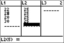
1. Enter the observed frequencies in $L1$ and the expected frequencies in $L2$.
2. Press 2nd [QUIT] to return to the home screen.
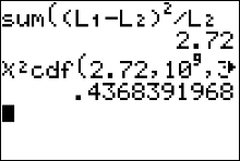
3. Press 2nd [LIST], move the cursor to MATH, and press 5 for sum(.
4. Type $(L1 - L2)^2/L2$, then press ENTER.

To calculate the P-value:
Press 2nd [DISTR] then press 7 to get $\chi^2 cdf($. (Use 8 on the TI-84)
For this P-value, the $\chi^2 cdf($ command has form $\chi^2 cdf($ test statistic, $10^9$ , degrees of freedom).
For this example use $\chi^2 \ cdf(2.72, \ 10^9, \ 3)$

---

An Easier Way to Get the Test Statistic and P-value

An alternative to using the Texas Instruments calculator is to use the Geogebra Probability Calculator on this web page link http://timbusken.com/prob-calc.html. Click on the distribution tab, then click on the Goodness of Fit Test. Afterwards enter the observed frequencies and the expected frequencies into the probability calculator. Once that is complete the calculator displays the values for the $df, $ the test statistic $ \chi^2$ and the $p-value$.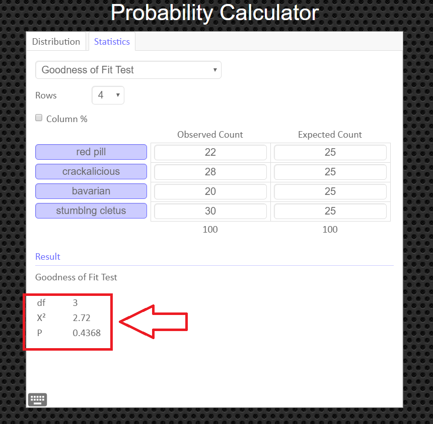

How to Obtain the Graph of the Chi-Square Distribution and P-value

Under the 'distribution' tab, click on 'Chi-Squared' Then enter in the degrees of freedom and the value of your test statistic, $\chi^2$, and click the '[' symbol (the left bracket symbol) to tell the calculator you have a right tailed test. You can export and save the graph as a png file if you need a copy of it to paste into your report.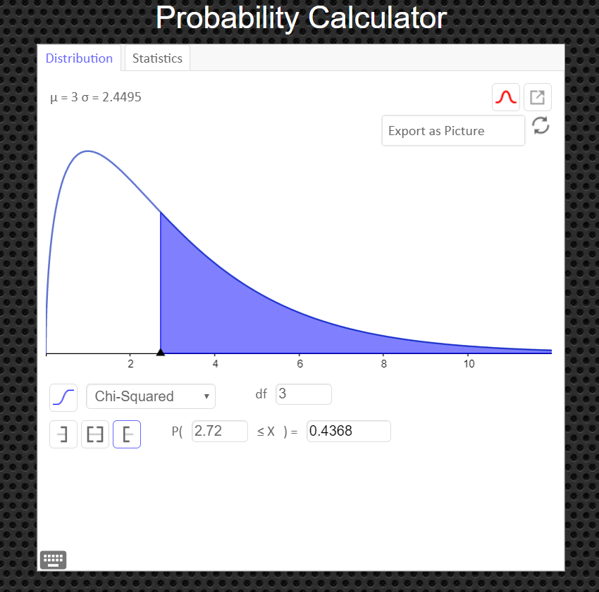

---

Example 2

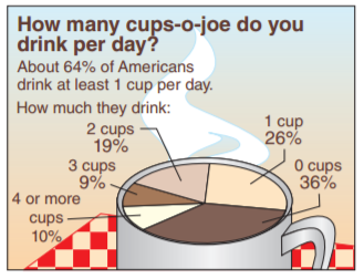
A researcher claims that the numbers of cups of coffee U.S. adults drink per day are distributed as shown in the figure. You randomly select 1600 U.S. adults and ask them how many cups of coffee they drink per day. The table shows the results. At $\alpha = 0.05$, test the researcher’s claim.

$$ \text{ Survey Results}\\ \begin{array}{c|c} Response & Frequency, f \\\hline 0 \text{ cups} & 570 \\ 1 \text{ cup} & 432 \\ 2 \text{ cups} & 282 \\ 3 \text{ cups} & 152 \\ 4 \text{ or more cups} & 164 \\ \end{array} $$

Solution

Step 1    State the null and alternative hypothesis.

Define the following population proportions: \[ \eqalign{ p_1 = & \text{the proportion of US adult who drink 0 cups per day} \cr p_2 = & \text{the proportion of US adult who drink 1 cups per day} \cr p_3 = & \text{the proportion of US adult who drink 2 cups per day} \cr p_4 = & \text{the proportion of US adult who drink 3 cups per day} \cr p_5 = & \text{the proportion of US adult who drink 4 or more cups per day} } \] Then the hypotheses are as follows: \[ \eqalign{ H_0: \quad & p_1 =36\%, \quad p_2 = 26\%, \quad p_3 =19\%, \quad p_4 =9\%, \quad p_5=10\% \cr H_a: \quad & \text{The distribution of the number of cups of coffee U.S. adults drink per day is different from the one given in the null hypothesis} } \]

Step 2    Find the value of your test statistic with the Chi-Square with the formula $\qquad\chi^2=\displaystyle\sum\frac{(O-E)^2}{E}$

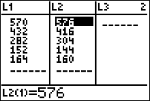
$$ \begin{array}{c|c|c} Response & Observed \ Frequency, O & Expected \ Frequency, E \\\hline 0 \text{ cups} & \color{red}{570} & 1600\cdot(0.36)=\color{blue}{576} \\ 1 \text{ cup} & \color{green}{432}& 1600\cdot(0.26)=\color{blue}{416} \\ 2 \text{ cups} & \color{orange}{282} & 1600\cdot(0.19)=\color{blue}{304}\\ 3 \text{ cups} & \color{red}{152} & 1600\cdot(0.09)=\color{blue}{144}\\ 4 \text{ or more cups} & \color{green}{164} & 1600\cdot(0.10)=\color{blue}{160}\\ \end{array} $$

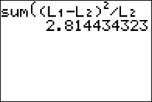
Then the test statistic value is \[ \eqalign{ \chi^2 & = \sum\frac{(O-E)^2}{E} \cr\cr & = \frac{( \color{red}{570}-\color{blue}{576})^2}{\color{blue}{576}}+ \frac{( \color{green}{432}-\color{blue}{416})^2}{\color{blue}{416}}+ \frac{( \color{orange}{282}-\color{blue}{304})^2}{\color{blue}{304}}+ \frac{( \color{red}{152}-\color{blue}{144})^2}{\color{blue}{144}}+ \frac{( \color{green}{164}-\color{blue}{160})^2}{\color{blue}{160}} \cr\cr & = 2.814 \qquad\text{ chi-square values are always rounded to the thousandths} } \]




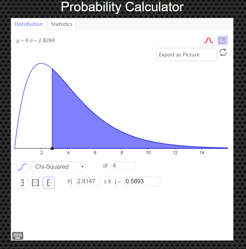
Step 3    Draw a picture of the Chi-Square Distribution (centered at df=number of categories minus1), and mark the location of your test statistic value along the x-axis in the right tail of your graph.



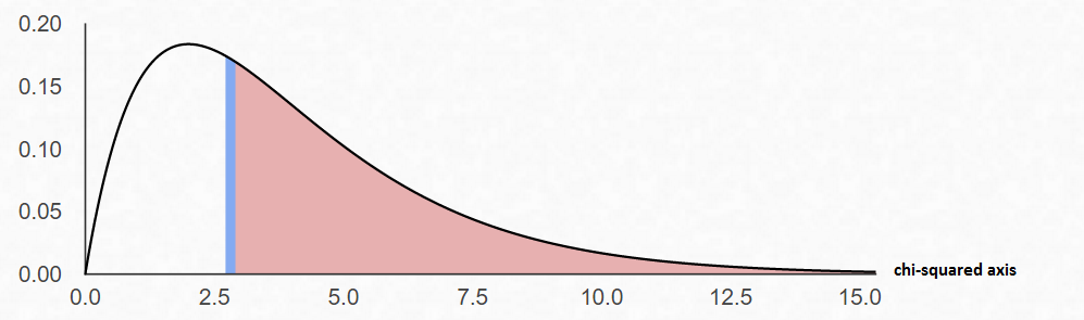
In the goodness-of-fit test, the degrees of freedom are equal to the number of categories minus 1. For this example, there are five categories; hence, the degrees of freedom are $5-1=4$. This is so because the number of subjects in each of the first three categories is free to vary. But in order for the sum to be 100 -- the total number of subjects -- the number of subjects in the last category is fixed.

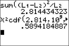
Step 4    Find the p-value. This will always be the area to the right of your test statistic. Find this value with your calculator's $\chi^2 \ cdf$ command. Use \[ \eqalign{ p-val & = \chi^2 \ cdf(\text{test stat value}, 10^9, \ df) \cr\cr & = \chi^2 \ cdf(2.814, \ 10^9, \ 4)\cr\cr & = 0.5894 } \]

Step 5    Use your p-value to make a decision about how to conclude the test.
We notice that $\alpha=0.05$ and the $p-val=0.5894$.
Since $p-val>\alpha$, fail to reject $H_0$ and conclude that the percentages are not significantly different from those given in the the claim.

How to Calculate the Test Statistic and P-Value

1. Enter the observed frequencies in $L1$ and the expected frequencies in $L2$.
2. Press 2nd [QUIT] to return to the home screen.
3. Press 2nd [LIST], move the cursor to MATH, and press 5 for sum(.
4. Type $(L1 - L2)^2/L2$, then press ENTER.

To calculate the P-value:
Press 2nd [DISTR] then press 7 to get $\chi^2 cdf($. (Use 8 on the TI-84)
For this P-value, the $\chi^2 cdf($ command has form $\chi^2 cdf($ test statistic, $10^9$ , degrees of freedom).
For this example use $\chi^2 \ cdf(2.814, \ 10^9, \ 4)$

An Easier Way to Get the Test Statistic and P-value

An alternative to using the Texas Instruments calculator is to use the Geogebra Probability Calculator on this web page link http://timbusken.com/prob-calc.html. Click on the distribution tab, then click on the Goodness of Fit Test. Afterwards enter the observed frequencies and the expected frequencies into the probability calculator. Once that is complete the calculator displays the values for the $df, $ the test statistic $ \chi^2$ and the $p-value$.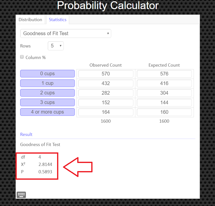

How to Obtain the Graph of the Chi-Square Distribution and P-value

Under the 'distribution' tab, click on 'Chi-Squared' Then enter in the degrees of freedom and the value of your test statistic, $\chi^2$, and click the '[' symbol (the left bracket symbol) to tell the calculator you have a right tailed test. You can export and save the graph as a png file if you need a copy of it to paste into your report.

---

---