Lab COVER SHEET
(click to download)
Definition
A correlation is a relationship between two variables. The data can be represented by the ordered pairs $(x, y)$, where $x$ is the independent (or explanatory) variable and $y$ is the dependent (or response) variable.
In an earlier chapter, you learned that the graph of ordered pairs $(x, y)$ is called a scatter plot. A scatter plot can be used to determine whether a linear (straight line) correlation exists between two variables. The scatter plots below show several types of correlation.
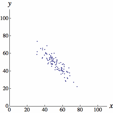
Negative Linear Correlation
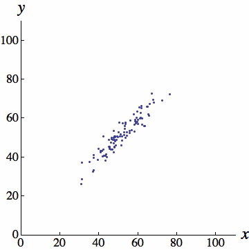
Strong Positive Linear Correlation
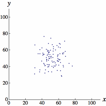
No Correlation
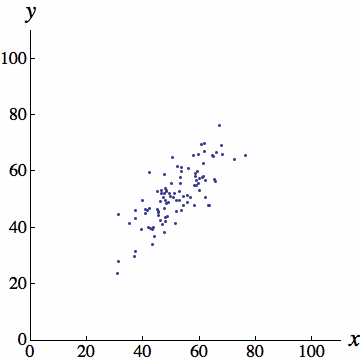
Moderate Positive Linear Correlation
(Images borrowed from Ken Kuniyuki)
Example (Fund Assets)
The table shows the total assets (in billions of dollars) of individual retirement accounts (IRAs) and federal pension plans for nine years.
| IRAs, $x$ | 2619 | 2533 | 2993 | 3299 | 3652 | 4207 | 4784 | 3585 | 4251 |
| Federal pension plans, $y$ | 860 | 894 | 958 | 1023 | 1072 | 1141 | 1197 | 1221 | 1324 |
Questions/Instructions
- Display the data in a scatter plot.
- Calculate the sample correlation coefficient, $r$.
- Describe the type of correlation.
- Interpret the correlation in the context of the data.
- Carry out the five steps of hypothesis testing and make a conclusion about the population correlation coefficient.
- Find the equation of the regression line for the data. Then construct the scatter plot and sketch the regression line with it.
-
Use the regression line equation to predict the value of $y$ for each $x$ value, if meaningful.
$ \begin{array}{ll} (a) & x=\$3000 \text{ billion}\\ (b) & x=\$5000 \text{ billion} \\ (c) & x= \$2500 \text{ billion}\\ (d) &x= \$10000 \text{ billion} \end{array} $ - Find the coefficient of determination, $r^2$. What does this tell you about the explained variation of the data about the regression line? About the unexplained variation?
- Find the standard error of estimate, $s_e$, needed to construct a prediction interval for the total assets in federal pension plans when the total assets in IRAs is $\$$3800 billion..
- Find the margin of error, $E$, needed to construct a 90% prediction interval for the total assets in federal pension plans when the total assets in IRAs is $\$$3800 billion.
- Construct a 90% prediction interval for the total assets in federal pension plans when the total assets in IRAs is $\$$3800 billion.
- Interpret the results.
Answers
- Display the data in a scatter plot.
To graph a scatter plot using the calculator:
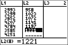
- Enter the x values in L1 and the y values in L2.
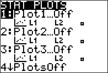
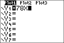
- Turn the calculator's [STAT PLOT] command on. Press the 2nd button followed by the $y=$ button to access Stat Plot 1. The other y functions should be turned off.
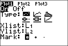
- Move the cursor to On and press ENTER on the Plot 1 menu.
- Move the cursor to the graphic that looks like a scatter plot next to Type (first graph), and press ENTER. Make sure the X list is L1, and the Y list is L2.
- Press GRAPH.
- Press ZOOM, followed by 9 (for the ZOOMSTAT command)
INPUT
INPUT
OUTPUT
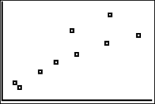
You can see that there is a positive linear correlation in the scatter plot. Unfortunately the calculator does not give you the numbers along the x and y axes.
- My calculator is having a syntax error!
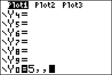
Press [1] to [QUIT]. If your calculator is throwing a syntax error, you need to turn the other y functions off. Press [y=] and clear out any function definitions with the CLEAR button.You may have to arrow down a bit to find the function definition that needs to be cleared out.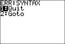
- My calculator is having a dim mismatch error!
Press [1] to [QUIT]. If your calculator is throwing a dim mismatch error, you probably have not entered in the same number of y values as x values. Open your list environment ([STAT] [ENTER]) and double check that you have entered in all of the data correctly.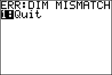
- Calculate the sample correlation coefficient, $r$.
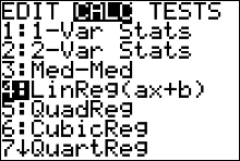
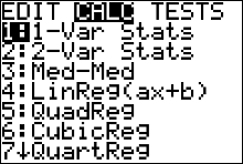
- Press STAT and move the cursor to Calc.
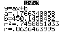
- Press 4 for LinReg(ax+b) then ENTER. The values for a, b, $r$ and $r^2$ will be displayed.
INPUT
INPUT
OUTPUT
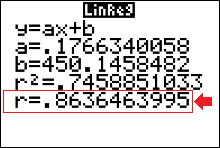
You can see that $r\approx 86\%$.
- My calculator does not give values for $r$ and $r^2$
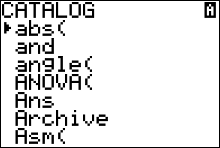
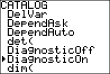
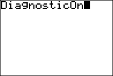
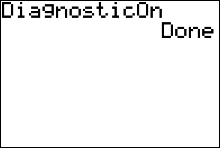
In order to have the calculator compute and display the correlation coefficient and coefficient of determination as well as the equation of the line, you must set the diagnostics display mode to on. Follow these steps:- Press 2nd then 0 for [CATALOG].
- Use the arrow keys to scroll down to DiagnosticOn.
- Press ENTER to copy the command to the home screen.
- Press ENTER to execute the command.
- Describe the type of correlation. There is a strong positive linear correlation between IRAs and Federal Pension Plans.
- Interpret the correlation in the context of the data. As IRA assets increase, the number of pension assets tends to increase.
- Carry out the five steps of hypothesis testing and make a conclusion about the population correlation coefficient.
We will conduct only two-tailed tests for $\rho$, the population correlation coefficient. As a result, for this type of test, the null and alternate hypotheses will always be \[ \eqalign{ H_0: \quad \rho=0& \quad\text{(no significant correlation)}\cr H_a: \quad \rho \neq 0 & \quad\text{(significant correlation)} } \] The standardized test statistic formula is \[ t=\dfrac{r}{\sqrt{\dfrac{1-r^2}{n-2}}} \approx 4.53 \text{ standard deviations} \] The pvalue $\approx0.0027$ (We can use the calculator to get this — see below). We use $\alpha=0.05$, since no value was given along with the statement of the problem. Since the p-value < $\alpha$, we reject the null hypothesis and conclude that there is a significant linear correlation between IRA assets and federal pension plan assets. (If we had instead obtained a pvalue that was greater than alpha, we would have not rejected the null hypothesis; and the conclusion would be that there is a NOT a significant linear correlation between IRA assets and federal pension plan assets.)
Since the correlation coefficient, $r$ was found to be significant in the hypothesis test above, the equation of the regression line can be determined. If, on the other, hand we did not reject the null hypothesis, then it would not be meaningful to calculate or use the regression line equation to make predictions.
We can use the calculator to obtain the pvalue and value of the standardized test statistic, $t$.
How to do a LinRegTTest
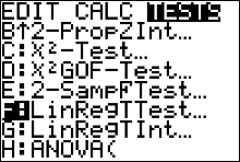
(to test the significance of $r$)- Press STAT and move the cursor to TESTS.
- Arrow down/up until your cursor is highlighting LinRegTTest. Then press ENTER.
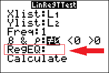
- Make sure the Xlist is L1, the Ylist is L2, and the Freq is 1.
- Select the $\neq$ for a two-tailed test.
- Leave blank or CLEAR the REGEQ.
(but if Y1 is already there, then leave it there) - Move the cursor to Calculate and press ENTER.
INPUT
INPUT
OUTPUT
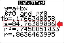
We obtain values for the standardized test statistic, $t$, and the pvalue. The small arrow at the bottom left corner of the output screen indicates that if you use your arrow down button you can see the rest of the output from the LinRegTTest.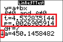
OUTPUT
- Find the equation of the regression line for the data. Then construct the scatter plot and sketch the regression line with it.
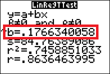
We can fetch the regression line equation from the output screens of the LinRegTTEst.
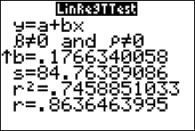
The calculator uses statistician's notation ($y=a+bx$) for the regression line equation. Notice the calculator gives you the specific values of $a$ and $b$. The regression line equation is then \[ \hat{y}=450.1458482 + 0.1766340052x \] Note that we use $\hat{y}$ (and not $y$) to describe the equation. This is because we could obtain a different regression line with a different sample from the same two populations. The variable $y$ is reserved (or used only) when we mean to talk about the regression line from the population. It is usually impossible to find the actual equation for $y$, but we can approximate it with a sample, which is what we are doing here.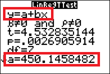
To plot the regression line on the scatter plot:
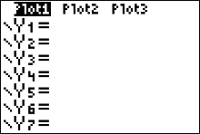
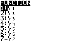
- Press the Y= button. Use the CLEAR button to delete all the equations appearing in your plots screen.
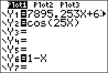
- Rerun the LinRegTTest but store Y1 as RegEq. Press [STAT] and move your cursor over to the TEST dropdown menu.
- Arrow down/up until your cursor is highlighting LinRegTTest. Then press ENTER.
INPUT
INPUT
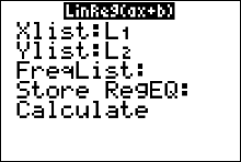
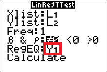
- Make sure that Xlist and Ylist are set to L1 and L2, and FreqList is cleared or left blank.
-
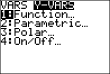
Move the cursor to Store RegEQ and press VARS and arrow over to the Y-VARS dropdown menu. Press ENTER (for Function) and ENTER again (for Y1). This should bring you back to the LinRegTTest input screen, and the regression equation will be stored as in the calculator as the function Y1.
INPUT
INPUT
INPUT
- Move your cursor to Calculate and press ENTER.
OUTPUT
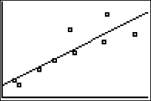
- Press GRAPH
OUTPUT
- Press the Y= button. Use the CLEAR button to delete all the equations appearing in your plots screen.
- Use the regression line equation to predict the value of $y$ for each $x$ value, if meaningful.
$ \begin{array}{ll} (a) & x=\$3,000 \text{ billion}\\ (b) & x=\$5,000 \text{ billion} \\ (c) & x= \$2,500 \text{ billion}\\ (d) &x= \$10,000 \text{ billion} \end{array} $
The regression equation is $\hat{y}=0.1766340052x+450.1458482$.
(a) When $x=\$3000 \text{ billion}$,
\[ \begin{array}{ll} \hat{y} &=0.1766340052x+450.1458482\\ &=0.1766340052(3000)+450.1458482 \\ &\approx \$980.05 \text{ billion} \end{array} \]
(b) When $x=\$5,000 \text{ billion}$,
\[ \begin{array}{ll} \hat{y} &=0.1766340052x+450.1458482\\ &=0.1766340052(5000)+450.1458482 \\ &\approx \$1,333.5 \text{ billion} \end{array} \]
(c) When $x=\$2,500 \text{ billion}$,
\[ \begin{array}{ll} \hat{y} &=0.1766340052x+450.1458482\\ &=0.1766340052(2500)+450.1458482 \\ &\approx \$891.73 \text{ billion} \end{array} \]
(d) When $x=\$10,000 \text{ billion}$, it is not meaningful to predict the value for $y$ because $x=\$10,000 \text{ billion}$ is far outside the range of the original data.
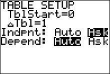
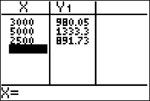
We could have our calculator evaluate the regression equation for us.- Press 2ND then WINDOW (to access TBLSET).
- The first two rows don’t matter. Move the cursor down to the Indpnt row. This controls the independent variable x.
- Move the cursor to Ask and press ENTER.
- Move the cursor to the Depend row highlight Auto and press ENTER.
- Now you can evaluate the function at selected x values. Press 2ND GRAPH. You may see some values on the table screen. They don’t do any harm, but if you want you can get rid of them by hitting DEL several times.
- Enter each x number and press ENTER. The TI-83/84 immediately displays the function value.
- Find the coefficient of determination, $r^2$. What does this tell you about the explained variation of the data about the regression line? About the unexplained variation?
You can get the coefficient of determination, $r^2$, from the output screen of either LinRegTTest or LinReg(ax+b).
The coefficient of determination, $r^2\approx0.746$.
74.6% of the variation in assets in federal pension plans can be explained by the relationship between IRA assets and federal pension plan assets, and 25.4% of the variation is unexplained.
- Find the standard error of estimate, $s_e$, needed to construct a prediction interval for the total assets in federal pension plans when the total assets in IRAs is $\$$3800 billion.
We can get the value for standard error when we do a LinRegTtest on the calculator (you will have to use the down arrow to find it). We find that $s_e\approx84.764$
- Find the margin of error, $E$, needed to construct a 90% prediction interval for the total assets in federal pension plans when the total assets in IRAs is $\$$3800 billion.
STEP 1 Identify that there are $n=9$ ordered pairs in the sample. Identify that $x_0=3800$.
STEP 2 Find $t_c$ using $n-2$ degrees of freedom.
Calculator: \[ \begin{array}{ll} t_c &=invT(area, df) \\ &=invT\biggr(\dfrac{1+c}{2}, \ n-2\biggr)\\ &= invT\biggr(\dfrac{1+0.90}{2},\ 9-2\biggr) \\ &=invT(0.95, \ 7)\approx1.895. \end{array} \]
$t$-table: The degrees of freedom are 7, so $t_c$ is on row 7 of the table. The area left of $t_c$ will be \[ \dfrac{1+c}{2}=\dfrac{1+0.90}{2}=0.95 \]Then, the column marked 95% intersects row 7 at the value 1.895, so $t_c\approx1.895$.
STEP 3 Find values for $\sum x, \ \ \sum x^2$ and $\bar{x}$ by running 1-var-stats on the data in list 1 (L1).
Press STAT and move your cursor to the TESTS dropdown menu. Press 1 (for 1-var-stats).
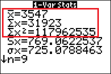
STEP 4 Evaluate the margin of error formula. \[ \begin{array}{ll} E &=t_c\cdot s_e\cdot\sqrt{1+\dfrac{1}{n}+\dfrac{n(x_0-\bar{x})^2}{n\cdot\sum x^2-(\sum x)^2}} \\[0.2in] &=(1.895)\cdot (84.764)\cdot\sqrt{1+\dfrac{1}{9}+\dfrac{9\cdot(3800-3547)^2}{9\cdot(117962535)-(31923)^2}} \\[0.2in] &=160.62778\cdot\sqrt{1+\dfrac{1}{9}+\dfrac{576081}{42584886}}\\[0.2in] &=160.62778\cdot\sqrt{1.124638939} \\[0.2in] &\approx170.344 \end{array} \] - Construct a 90% prediction interval for the total assets in federal pension plans when the total assets in IRAs is $\$$3800 billion.
The point estimate is \[ \hat{y}=0.1766340052\cdot(3800)+450.1458482\approx1121.4 \] or $\$1,121,400,000$.
The interval estimate for $y$ when $x=\$3,800,000,000,000$ \[ \hat{y}-E < y < \hat{y}+E \] \[ 1121.4-170.344 < y < 1121.4+170.344 \] \[ 951.056 \text{ billion}< y < 1291.744 \text{ billion} \] \[ \$951,056,000,000 < y < \$1,291,744,000,000 \] - Interpret the results.
Types of Variation
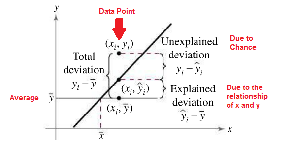
The total variation $\sum(y_i-\bar{y})^2$ is the sum of the squares of the vertical distances each
point is from the mean. The total variation can be divided into two parts: that which is
attributed to the relationship of $x$ and $y$ and that which is due to chance. The variation
obtained from the relationship (i.e., from the predicted $\hat{y_i}$ values) is $\sum(\hat{y_i}-\bar{y})^2$ and is
called the explained variation. Most of the variations can be explained by the relationship.
The closer the value $r$ is to -1 or 1, the better the points fit the line and the closer
$\sum(\hat{y_i}-\bar{y})^2$ is to $\sum(y_i-\bar{y})^2$. In fact, if all points fall on the regression line, $\sum(\hat{y_i}-\bar{y})^2$ will
equal $\sum(y_i-\bar{y})^2$, since $\bar{y}$ is equal to $y$ in each case.
On the other hand, the variation due to chance, found by $\sum(y_i-\hat{y_i})^2$, is called the
unexplained variation. This variation cannot be attributed to the relationship. When
the unexplained variation is small, the value of $r$ is close to -1 or 1. If all points fall on
the regression line, the unexplained variation $\sum(y_i-\hat{y_i})^2$ will be 0. Hence, the total variation
is equal to the sum of the explained variation and the unexplained variation. That is,
$\sum(y_i-\bar{y_i})^2 = \sum(\hat{y_i}-\bar{y})^2 + \sum(y_i-\hat{y_i})^2$
These values are shown in the figure above. For a single point, the differences are called deviations.
The values $y-\hat{y}$ are called residuals. A residual is the difference between
the actual value of y and the predicted value $\hat{y}$ for a given $x$ value. The mean of the residuals
is always zero. As stated previously, the regression line determined by the formulas
given in the textbook is the line that best fits the points of the scatter plot. The sum of the
squares of the residuals computed by using the regression line is the smallest possible
value. For this reason, a regression line is also called a least-squares line.
Coefficient of Determination
The coefficient of determination is the ratio of the explained variation to the total variation and is denoted by $r^2$. That is, \[ r^2=\frac{\text{explained variation}}{\text{total variation}} \] The term $r^2$ is usually expressed as a percentage. Another way to arrive at the value for $r^2$ is to square the correlation coefficient.Definition
The coefficient of determination is a measure of the variation of the dependent variable that is explained by the regression line and the independent variable. The symbol for the coefficient of determination is $r^2$.
Of course, it is usually easier to find the coefficient of determination by squaring $r$ and converting it to a percentage. Therefore, if $r = 0.90$, then $r^2 = 0.81$, which is equivalent to 81%. This result means that 81% of the variation in the dependent variable is accounted for by the variations in the independent variable. The rest of the variation, 0.19, or 19%, is unexplained. This value is called the coefficient of nondetermination and is found by subtracting the coefficient of determination from 1. As the value of $r$ approaches 0, $r^2$ decreases more rapidly. For example, if $r = 0.6$, then $r^2 = 0.36$, which means that only 36% of the variation in the dependent variable can be attributed to the variation in the independent variable.
Definition
Coefficient of Nondetermination \[1-r^2\]
Standard Error of the Estimate
When a $\hat{y}$ value is predicted for a specific $x$ value, the prediction is a point prediction. However, a prediction interval about the value can be constructed, just as a confidence interval was constructed for an estimate of the population mean. The prediction interval uses a statistic called the standard error of the estimate.Definition
The standard error of the estimate, denoted by $s_e$, is the standard deviation of the observed $y_i$ values about the $\hat{y}$ predicted values. The formula for the standard error of the estimate is \[ s_e = \sqrt{\frac{\sum(y_i-\hat{y_i})^2}{n-2}} \] where $n$ is the number of pairs of data.
The standard error of the estimate is similar to the standard deviation, but the mean is not used. As can be seen from the formula, the standard error of the estimate is the square root of the unexplained variation—that is, the variation due to the difference of the observed values and the expected values—divided by $n - 2$. So the closer the observed values are to the predicted values, the smaller the standard error of the estimate will be.
Prediction Intervals
The standard error of the estimate can be used for constructing a prediction interval (similar to a confidence interval) about a $\hat{y}$ value.When a specific value $x$ is substituted into the regression equation, the $\hat{y}$ that you get is a point estimate for $y$. For example, the regression line equation for the amount in IRAs and federal pension plans is $\hat{y}=0.1766340052x+450.1458482$, then the predicted amount in federal pension plans when the amount in IRAs is $\$$3800 billion would be \[ \hat{y}=0.1766340052\cdot(3800)+450.1458482\approx1121.4 \] or $\$1,121,400,000$. Since this is a point estimate, you have no idea how accurate it is. But you can construct a prediction interval about the estimate. By selecting an a level of confidence, $c$, you can achieve $c$% confidence that the interval contains the actual mean of the $y$ values that correspond to the given value of $x$.
The reason is that there are possible sources of prediction errors in finding the regression line equation. One source occurs when finding the standard error of the estimate $s_e$. Two others are errors made in estimating the slope and the $\hat{y}$ intercept, since the equation of the regression line will change somewhat if different random samples are used when calculating the equation.
$c$-Prediction Interval
Given a linear regression equation $\hat{y}=mx+b$ and $x_0$, a specific value of $x$, a $c$-prediction interval for $y$ is \[ \hat{y}-E < y < \hat{y}+E \] where \[ E=t_c\cdot s_e\cdot\sqrt{1+\frac{1}{n}+\frac{n(x_0-\bar{x})^2}{n\cdot\sum x^2-(\sum x)^2}} \] and the degrees of freedom used to find $t_c$ are $df=n-2$, with $n$ being equal to the number of pairs of data in the sample. The point estimate is $\hat{y}$ and the margin of error is $E$. The probability that the prediction interval contains $y$ is $c$ (the level of confidence), assuming that the estimation process is repeated a large number of times.
You can be 90% confident that the total assets of federal pension plans will be between $\$951,056,000,000$ and $\$1,291,744,000,000$ when the total assets of IRAs is $\$3,800,000,000,000$.