Test for Independence
The chi-square independence test can be used to test the independence of two variables. Using this test, you can determine whether the occurrence of one variable affects the probability of the occurrence of the other variable. Before performing a chi-square independence test, you must verify that (1) the observed frequencies were obtained from a random sample and (2) each expected frequency is at least 5.Suppose for example, a researcher wishes to determine whether there is a relationship between the gender of an individual and the amount of alcohol consumed. A sample of 68 people is selected, and the following data are obtained. $$ \qquad\quad \underline{Alcohol \ Consumption}\\ \begin{array}{c|c|c|c} Gender & Low & Moderate & High \\\hline Male & 10 & 9 & 8 \\ Female & 13 & 16 & 12 \\ \end{array} $$ At $\alpha=0.10$, can the researcher conclude that alcohol consumption is related to gender?
The correct hypotheses are:
$ H_0: \qquad $The amount of alcohol that a person consumes is independent of the individual’s gender.
$H_a: \qquad $ The amount of alcohol that a person consumes is dependent on the individual’s gender (claim).
When data are arranged in table form for the chi-square independence test, the table is called a contingency table. The table is made up of R rows and C columns. The table here has two rows and three columns. Note that row and column headings do not count in determining the number of rows and columns.
A contingency table is designated as an $R \times C$ (rows by columns) table. In this case, $R = 2$ and $C =3$; hence, this table is a $2 \times 3$ (2 by 3) contingency table. Each block in the table is called a cell and is designated by its row and column position. For example, the cell with a frequency of 9 is designated as $C_{1,2}$, or row 1, column 2. The cells are shown below.
$$ \begin{array}{c|c|c|c} & Column \ 1 & Column \ 2 & Column \ 3 \\\hline row \ 1 & C_{1,1} & C_{1,2} & C_{1,3} \\ row \ 2 & C_{2,1} & C_{2,2} & C_{2,3} \\ \end{array} $$
The degrees of freedom for any contingency table are (number of rows - 1) times (number of columns - 1); that is, \[ df = (R - 1)\cdot(C - 1). \] In this case, $(2 - 1)\cdot(3 - 1) = (1)\cdot(2) = 2$. The reason for this formula for d.f. is that all the expected values except one are free to vary in each row and in each column.
Definition
$$ \qquad\quad \underline{\color{blue}{Alcohol \ Consumption}}\\ \begin{array}{c|c|c|c|c} \color{blue}{Gender} & Low & Moderate & High & Row \ Totals \\\hline Male & 10 & 9 & 8 & 27\\ Female & 13 & 16 & 12 & 41\\ \hline \quad Column \ Totals &23&25&20&68\\ \end{array} $$
When you find the sum of each row and column in a contingency table, you are calculating the marginal frequencies. A marginal frequency is the frequency that an entire category of one of the variables occurs. For instance, in the table above, the marginal frequency for subjects whose consumption is low 10 + 13 = 23. The observed frequencies in the interior of a contingency table are called joint frequencies.
CAUTION: Sometimes the statement of the problem will give you the contingency table along with the marginal frequencies. Whenever they do this, DO NOT include row and column totals when counting the number of rows and columns in the table to find degrees of freedom. For example, the table directly above this includes marginal frequencies, however the table is still a 2 by 3 contingency table.
Finding the Expected Frequency, E, for Contingency Table Cells
For our example problem, since we have 6 observed frequencies, we will have six expected frequencies. We will have to use the formula six times, as follows.
$$ \qquad\quad \underline{\color{blue}{Alcohol \ Consumption}}\\ \begin{array}{c|c|c|c|c} \color{blue}{Gender} & Low & Moderate & High & Row \ Totals \\\hline Male & 10 & 9 & 8 & 27\\ Female & 13 & 16 & 12 & 41\\ \hline \quad Column \ Totals &23&25&20&68\\ \end{array} $$
\[ E_{1,1}=\frac{27\cdot23}{68}=9.132352941 \qquad E_{1,2}=\frac{27\cdot25}{68}=9.926470588 \qquad E_{1,3}=\frac{27\cdot20}{68}=7.941176471 \] \[ E_{2,1}=\frac{41\cdot23}{68}=13.86764706 \qquad E_{2,2}=\frac{41\cdot25}{68}=15.07352941 \qquad E_{2,3}=\frac{41\cdot20}{68}=12.05882353 \]
The Chi-Square Independence Test
- State the null and alternative hypotheses. Identify which one is the claim. The null will be a statement saying the two variables are independent. The alternate will say they are dependent.
- Find the value of your test statistic with the Chi-Square with the formula
\[
\chi^2=\displaystyle\sum\frac{(O-E)^2}{E}
\]
First though, you have to find the expected frequency for each cell with the formula
\[
E= \frac{\text{(row total)}\cdot\text{(column total)}}{\text{sample size}}
\]
- Draw a picture of the Chi-Square Distribution, centered at $df=(R-1)\cdot(C-1)$, and mark the location of your test statistic value along the x-axis in the right tail of your graph.
- Find the p-value. This will always be the area to the right of your test statistic. Find this value with your calculator's $\chi^2 \ cdf$ command. Use
\[
\chi^2 \ cdf(\text{test stat value}, 10^9, \ df) \qquad\text{with $df=(R-1)\cdot(C-1)$}
\]
- Use your p-value to make a decision about how to conclude the test.
- If the $p-val\leq\alpha$, reject $H_0$ and conclude that the sample evidence suggests that the variables are dependent (related).
- If the $p-val>\alpha$, fail to reject $H_0$, and conclude that the sample evidence suggests that the variables are independent (not related).
Assumptions:
- The data are obtained from a random sample.
- The expected frequency for each category must be 5 or more.
The expected frequencies are calculated on the assumption that the two
variables are independent. If the variables are independent, then you can expect
little difference between the observed frequencies and the expected frequencies.
When the observed frequencies closely match the expected frequencies, the
differences between O and E will be small and the chi-square test statistic will be
close to 0. As such, the null hypothesis is unlikely to be rejected.
For dependent variables, however, there will be large discrepancies between
the observed frequencies and the expected frequencies. When the differences
between O and E are large, the chi-square test statistic is also large. A large
chi-square test statistic is evidence for rejecting the null hypothesis. So, the
chi-square independence test is always a right-tailed test
Example 1
Suppose for example, a researcher wishes to determine whether there is a relationship between the gender of an individual and the amount of alcohol consumed. A sample of 68 people is selected, and the following data are obtained. $$ \qquad\quad \underline{Alcohol \ Consumption}\\ \begin{array}{c|c|c|c} Gender & Low & Moderate & High \\\hline Male & 10 & 9 & 8 \\ Female & 13 & 16 & 12 \\ \end{array} $$ At $\alpha=0.10$, can the researcher conclude that alcohol consumption is related to gender?Solution
Step 1 State the null and alternative hypothesis. Identify which one is the claim, if a claim is mentioned in the statement of the problem.$ H_0: \qquad $The amount of alcohol that a person consumes is independent of the individual’s gender.
$H_a: \qquad $ The amount of alcohol that a person consumes is dependent on the individual’s gender (claim).
Step 2 Find the value of your test statistic $\chi^2$, but first find each expected frequency.
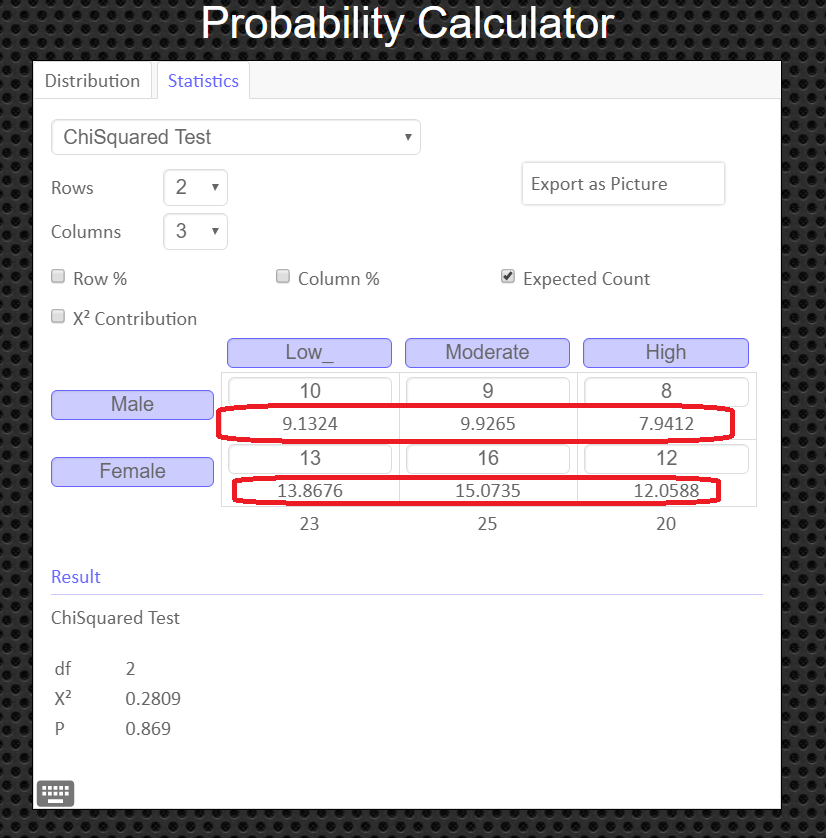
We did this above. The completed table is below. Each expected frequency, E, is next to each observed frequency, O, in parenthesis. $$ \qquad\quad \underline{\color{blue}{Alcohol \ Consumption}}\\ \begin{array}{c|c|c|c|c} \color{blue}{Gender} & Low & Moderate & High & Row \ Totals \\\hline Male & 10 \ (9.132352941) & 9 \ (9.926470588) & 8 \ (7.941176471) & 27\\ Female & 13 \ (13.86764706) & 16 \ (15.07352941) & 12 \ (12.05882353)& 41\\ \hline \quad Column \ Totals &23&25&20&68\\ \end{array} $$
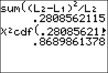
The test statistic is \[ \eqalign{ \chi^2 & = \sum\frac{(O-E)^2}{E} \cr\cr & = \frac{ (10-9.132352941)^2}{9.132352941}+ \frac{ (9-9.926470588)^2}{9.926470588}+ \frac{ (8-7.941176471)^2}{7.941176471} \cr\cr & \qquad + \frac{ (13-13.86764706)^2}{13.86764706}+ \frac{ (16-15.07352941)^2}{15.07352941}+ \frac{ (12-12.05882353)^2}{12.05882353} \cr\cr & = 0.2808562115 } \] We can have the calculator find this value for us the same way we did in Section 10.1 (see instruction below)
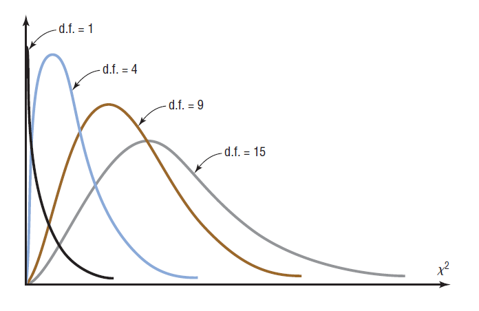
Step 3 Draw a picture of the Chi-Square Distribution (centered at $df=(R-1)\cdot(C-1)$), and mark the location of your test statistic value along the x-axis in the right tail of your graph.
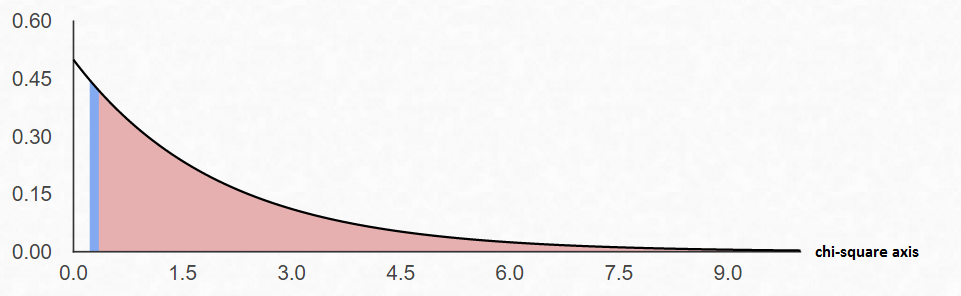
Step 4 Find the p-value. This will always be the area to the right of your test statistic. Find this value with your calculator's $\chi^2 \ cdf$ command. Use \[ \eqalign{ p-val & = \chi^2 \ cdf(\text{test stat value}, 10^9, \ df) \cr\cr & = \chi^2 \ cdf(0.2808562115, \ 10^9, \ 2)\cr\cr & = 0.8689861378 } \] Step 5 Use your p-value to make a decision about how to conclude the test.
We notice that $\alpha=0.10$ and the $p-val=0.8690$ (rounded to the ten-thousandths).
Since $p-val>\alpha$, fail to reject $H_0$ and conclude that the sample evidence suggests that the variables are independent.
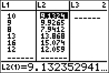
How to Calculate the Test Statistic and P-Value
- Enter the observed frequencies in $L1$ and the expected frequencies in $L2$.
- Press 2nd [QUIT] to return to the home screen.
- Press 2nd [LIST], move the cursor to MATH, and press 5 for sum(.
- Type $(L1 - L2)^2/L2$, then press ENTER.
To calculate the P-value:
Press 2nd [DISTR] then press 7 to get $\chi^2 cdf($. (Use 8 on the TI-84)
For this P-value, the $\chi^2 cdf($ command has form $\chi^2 cdf($ test statistic, $10^9$ , degrees of freedom).
For this example use $\chi^2 \ cdf(0.2808562115, \ 10^9, \ 2)$
An Easier Way to Get the Test Statistic and P-value
An alternative to using the Texas Instruments calculator is to use the Geogebra Probability Calculator on this web page link http://timbusken.com/prob-calc.html. Click on the distribution tab, then click on the ChiSquared Test. Afterwards enter the contingency table into the probability calculator. Once that is complete the calculator displays the values for the $df, \chi^2$ and the pvalue.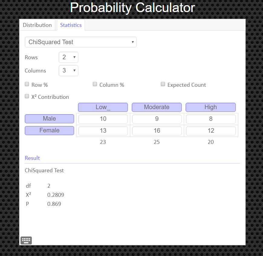
If you need to see values for the expected frequencies, click on the box labeled 'Expected Count'.
How to Obtain the Graph of the Chi-Square Distribution and P-value
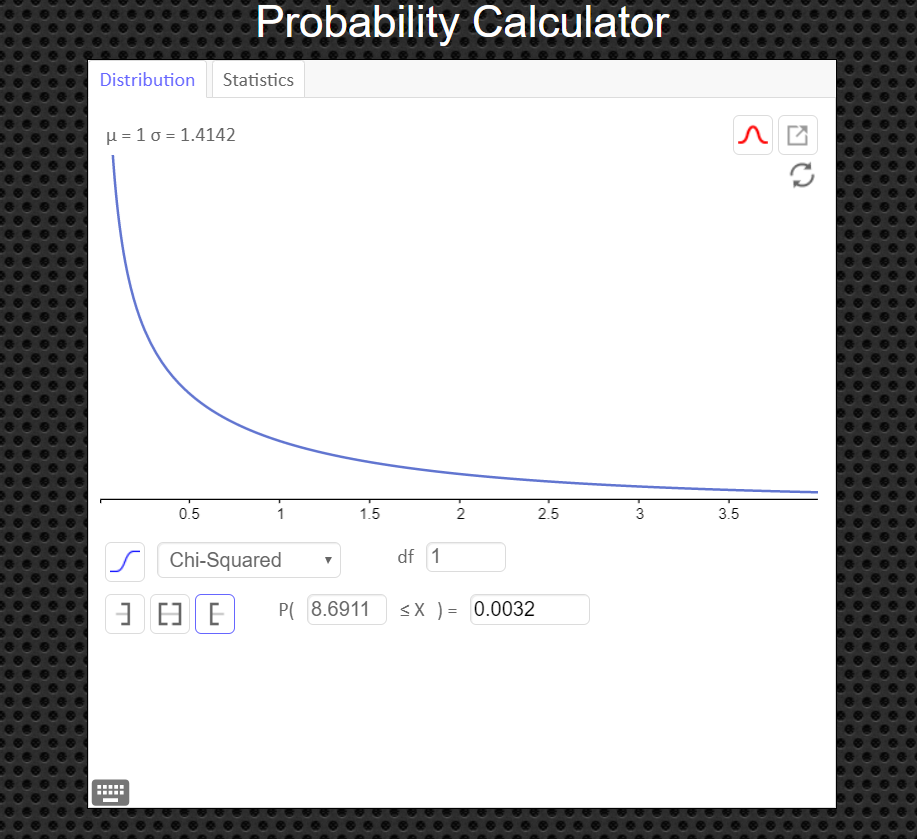
Under the 'distribution' tab, click on 'Chi-Squared' Then enter in the degrees of freedom and the value of your test statistic, $\chi^2$, and click the '[' symbol (the left bracket symbol) to tell the calculator you have a right tailed test. You can export and save the graph as a png file if you need a copy of it to paste into your report.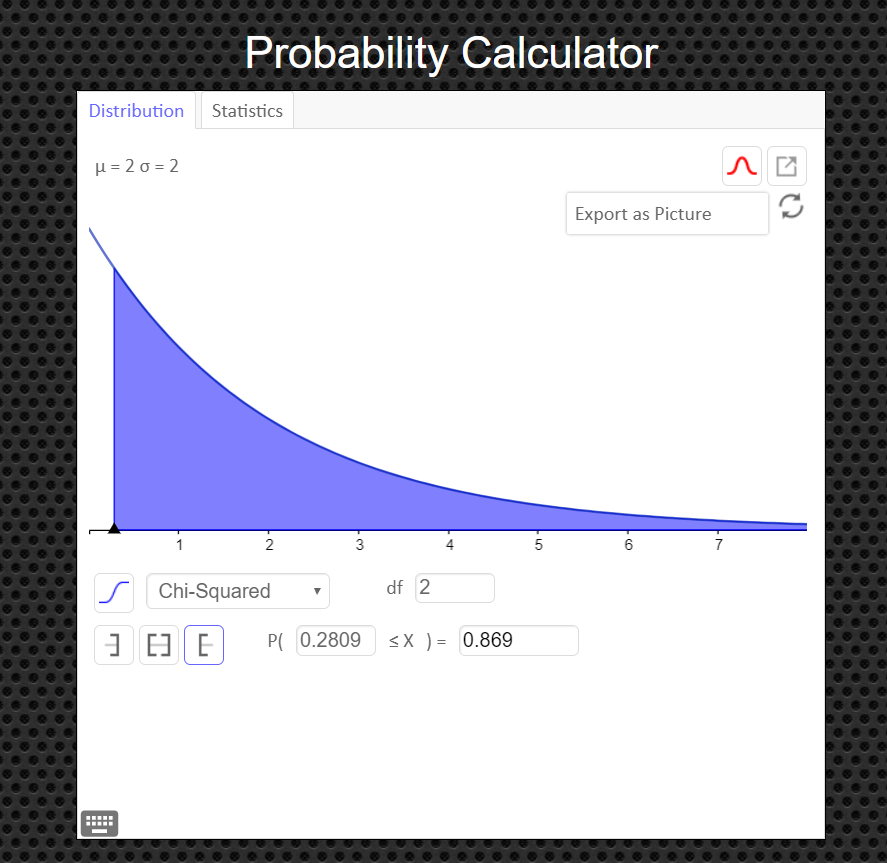
Example 2
Attitudes about Safety The contingency table shows the results of a random sample of students by type of school and their attitudes on safety steps taken by the school staff. $$ \qquad\qquad \text{School staff has}\\ \begin{array}{c|c|c|c} \text{Type of} & \text{Taken all steps necessary} & \text{Taken some steps}\\ \text{School} & \text{for student safety} & \text{toward student safety} \\\hline \text{Public} & 40 & 51\\ \text{Private} & 64 & 34 \\ \end{array} $$ At $\alpha = 0.01$, can you conclude that attitudes about the safety steps taken by the school staff are related to the type of school?Solution
Step 1 State the null and alternative hypothesis. Identify which one is the claim, if a claim is mentioned in the statement of the problem.$ H_0: \qquad $Attitudes about safety are independent of the type of school.
$H_a: \qquad $ Attitudes about safety are dependent of the type of school (claim).
Step 2 Find the value of your test statistic $\chi^2$, but first find each expected frequency.
We begin this step by finding marginal frequencies (row and column totals). $$ \qquad\qquad \text{School staff has}\\ \begin{array}{c|c|c|c|c} \text{Type of} & \text{Taken all steps necessary} & \text{Taken some steps}&\\ \text{School} & \text{for student safety} & \text{toward student safety} & \text{row total}\\\hline \text{Public} & 40 & 51&91\\ \text{Private} & 64 & 34&98 \\\hline \text{column total}&104&85&189 \end{array} $$
Then we use the formula to find all the expected frequencies: \[ \text{Expected Frequency } E_{r,c}= \frac{\text{(row total)}\cdot\text{(column total)}}{\text{sample size}} \]
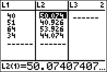
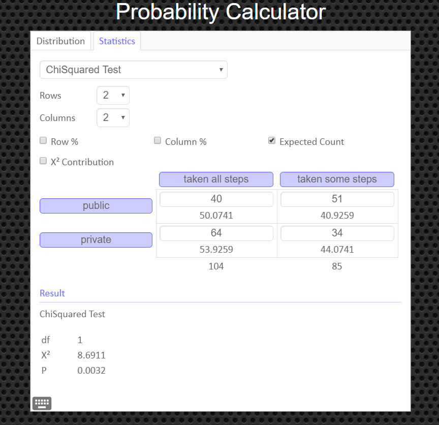
\[ E_{1,1}=\frac{91\cdot104}{189}=50.07407407 \qquad E_{1,2}=\frac{91\cdot85}{189}=40.92592593 \] \[ E_{2,1}=\frac{98\cdot104}{189}=53.92592593 \qquad E_{2,2}=\frac{98\cdot85}{189}=44.07407407 \]
The completed table is below. Each expected frequency, E, is next to each observed frequency, O, in parenthesis.
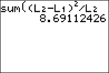
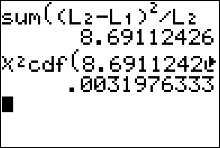
$$ \qquad\qquad \text{School staff has}\\ \begin{array}{c|c|c|c|c} \text{Type of} & \text{Taken all steps necessary} & \text{Taken some steps}&\\ \text{School} & \text{for student safety} & \text{toward student safety} & \text{row total}\\\hline \text{Public} & 40 (50.07407407) & 51 (40.92592593)&91\\ \text{Private} & 64 (53.92592593) & 34 (44.07407407)&98 \\\hline \text{column total}&104&85&189 \end{array} $$ The test statistic is \[ \eqalign{ \chi^2 & = \sum\frac{(O-E)^2}{E} \cr\cr & = \frac{ (40-50.07407407)^2}{50.07407407}+ \frac{ (51-40.92592593)^2}{40.92592593} + \frac{ (64-53.92592593)^2}{53.92592593} + \frac{ (34-44.07407407)^2}{44.07407407} \cr\cr & = 8.69112426 \qquad\text{ chi-square values are always rounded to the thousandths} } \]
Step 3 Draw a picture of the Chi-Square Distribution (centered at $df=(R-1)\cdot(C-1)$), and mark the location of your test statistic value along the x-axis in the right tail of your graph.
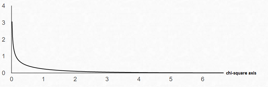
Step 4 Find the p-value. This will always be the area to the right of your test statistic. Find this value with your calculator's $\chi^2 \ cdf$ command. Use \[ \eqalign{ p-val & = \chi^2 \ cdf(\text{test stat value}, 10^9, \ df) \cr\cr & = \chi^2 \ cdf(8.69112426, \ 10^9, \ 1)\cr\cr & = 0.0031976333 } \]
Step 5 Use your p-value to make a decision about how to conclude the test.
We notice that $\alpha=0.10$ and the $p-val=0.0032$ (rounded to the ten-thousandths).
Since $p-val\leq\alpha$, reject $H_0$. The sample data suggests the variables are dependent.
How to Calculate the Test Statistic and P-Value
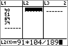
- Enter the observed frequencies in $L1$ and the expected frequencies in $L2$.
- Press 2nd [QUIT] to return to the home screen.
- Press 2nd [LIST], move the cursor to MATH, and press 5 for sum(.
- Type $(L1 - L2)^2/L2$, then press ENTER.
To calculate the P-value:
Press 2nd [DISTR] then press 7 to get $\chi^2 cdf($. (Use 8 on the TI-84)
For this P-value, the $\chi^2 cdf($ command has form $\chi^2 cdf($ test statistic, $10^9$ , degrees of freedom).
For this example use $\chi^2 \ cdf(8.69112426, \ 10^9, \ 1)$
An Easier Way to Get the Test Statistic and P-value
An alternative to using the Texas Instruments calculator is to use the Geogebra Probability Calculator on this web page link http://timbusken.com/prob-calc.html. Click on the distribution tab, then click on the ChiSquared Test. Afterwards enter the contingency table into the probability calculator. Once that is complete the calculator displays the values for the $df, \chi^2$ and the pvalue.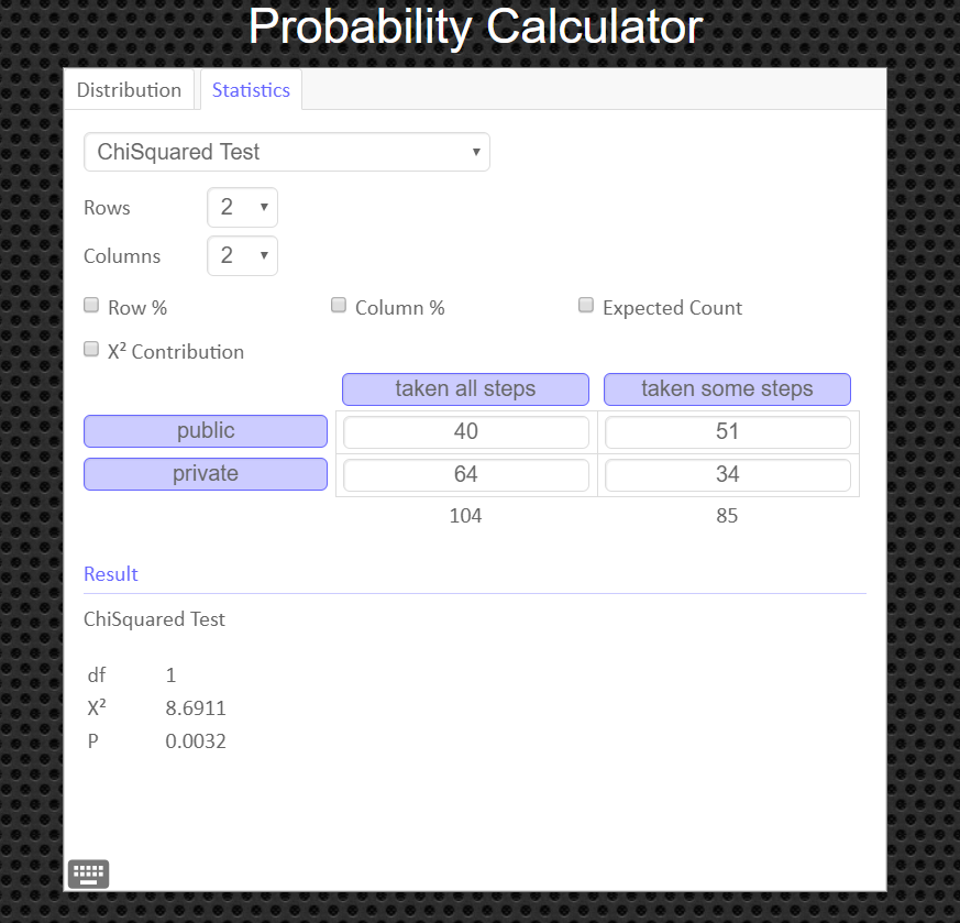
If you need to see values for the expected frequencies, click on the box labeled 'Expected Count'.
How to Obtain the Graph of the Chi-Square Distribution and P-value
Under the 'distribution' tab, click on 'Chi-Squared' Then enter in the degrees of freedom and the value of your test statistic, $\chi^2$, and click the '[' symbol (the left bracket symbol) to tell the calculator you have a right tailed test. You can export and save the graph as a png file if you need a copy of it to paste into your report.